Lecture 2. Visual Vocabulary & Effective Visualizations
PUBH 6199: Visualizing Data with R, Summer 2025
2025-05-27
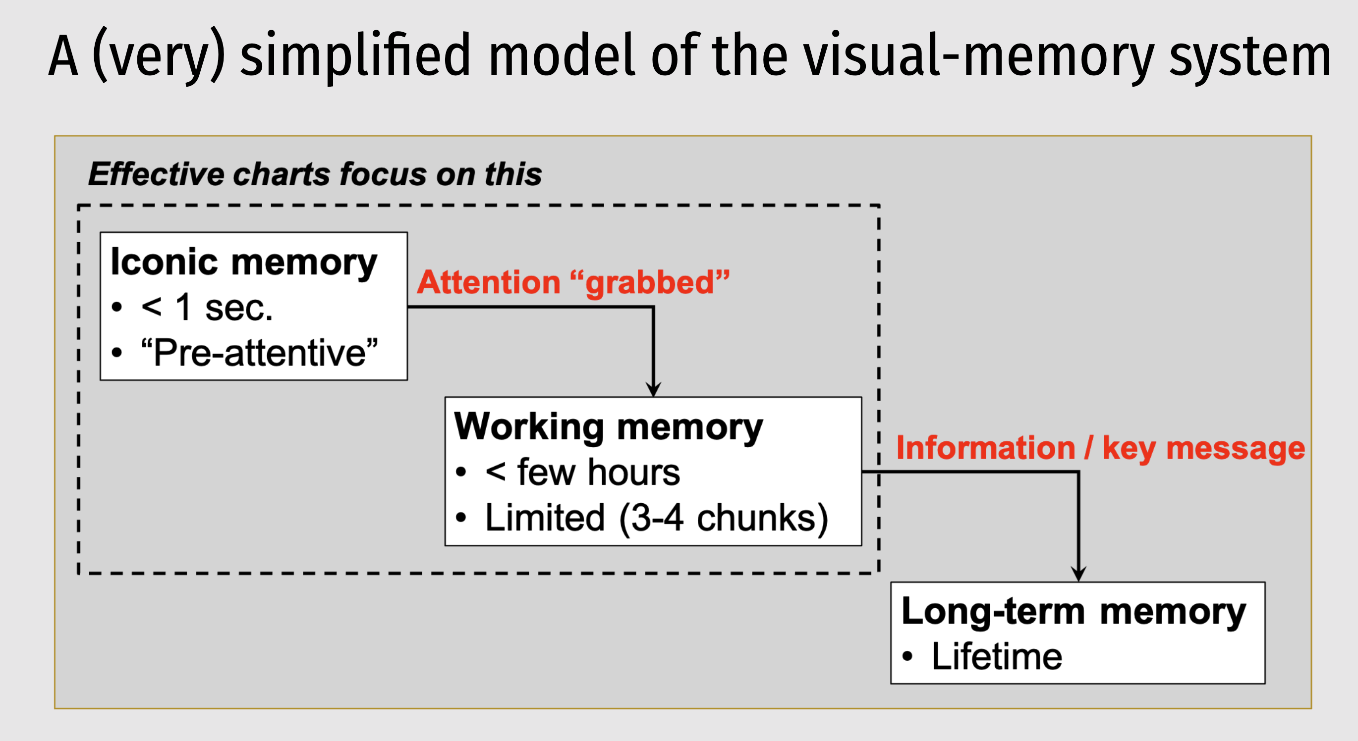
Good data visualization is optimized for our visual-memory system
Helps us understand trends and patterns
Makes data more accessible to different audiences
Useful in decision-making and communication
The power of pre-attentive processing
Count all the 5s in the following image
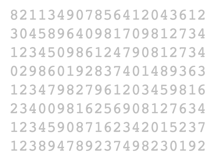
The power of pre-attentive processing
Count all the 5s in the following image
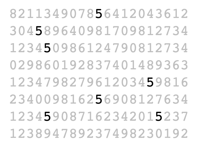
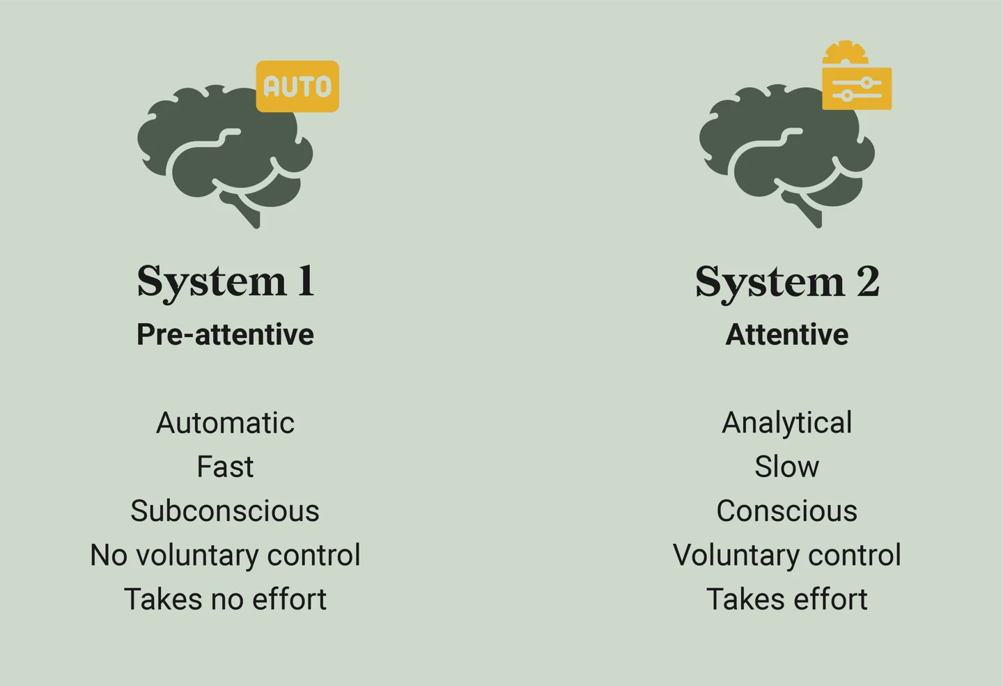
What is pre-attentive processing?
- Rapid, automatic processing of visual information before conscious attention kicks in.
- Happens within <250 milliseconds.
- Helps identify key patterns without effort.
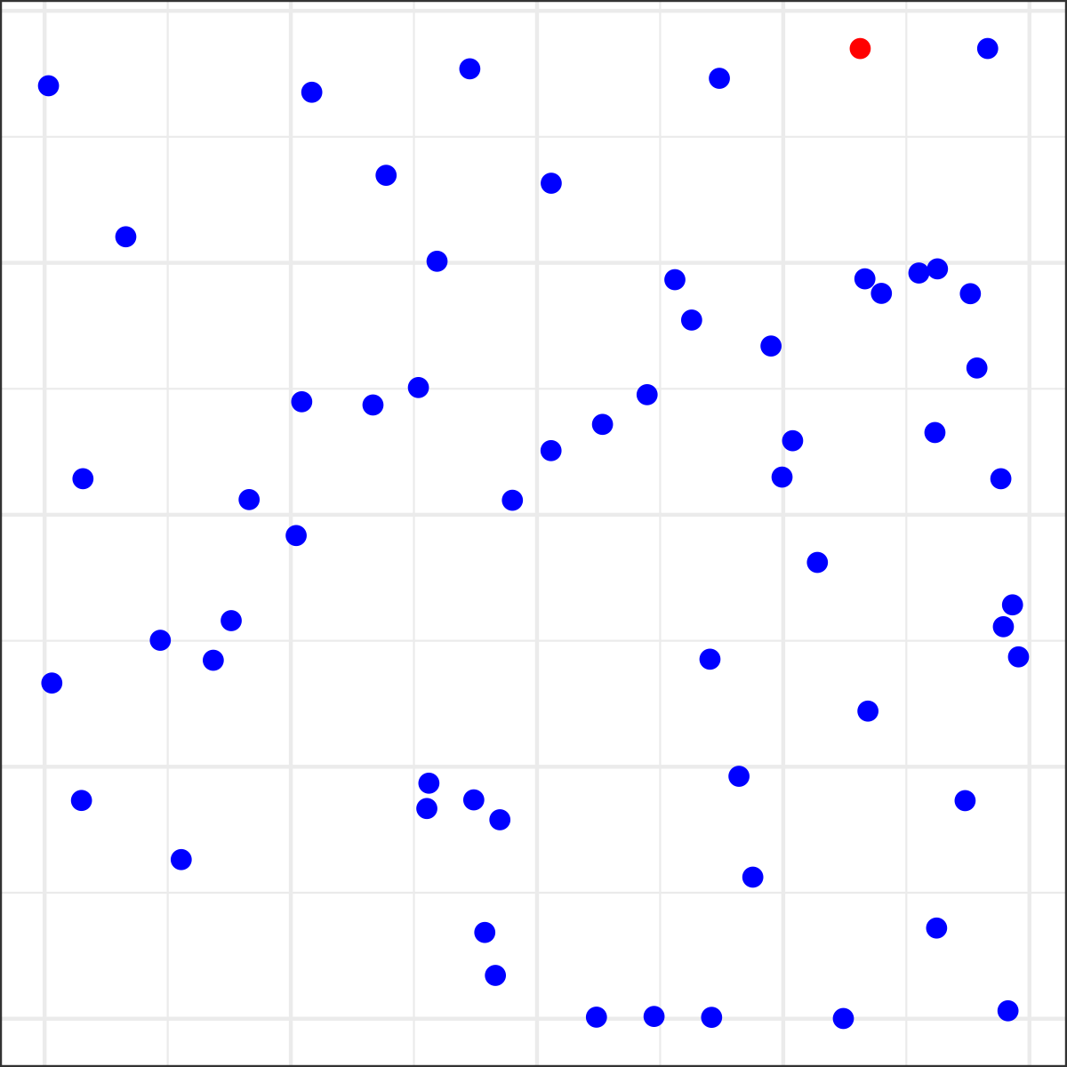
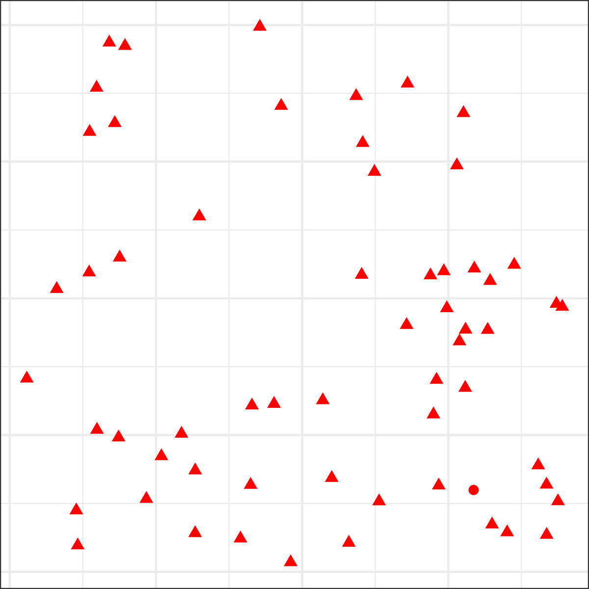
Not all pre-attentive features are created equal
Raise your hand when you see the red dot?
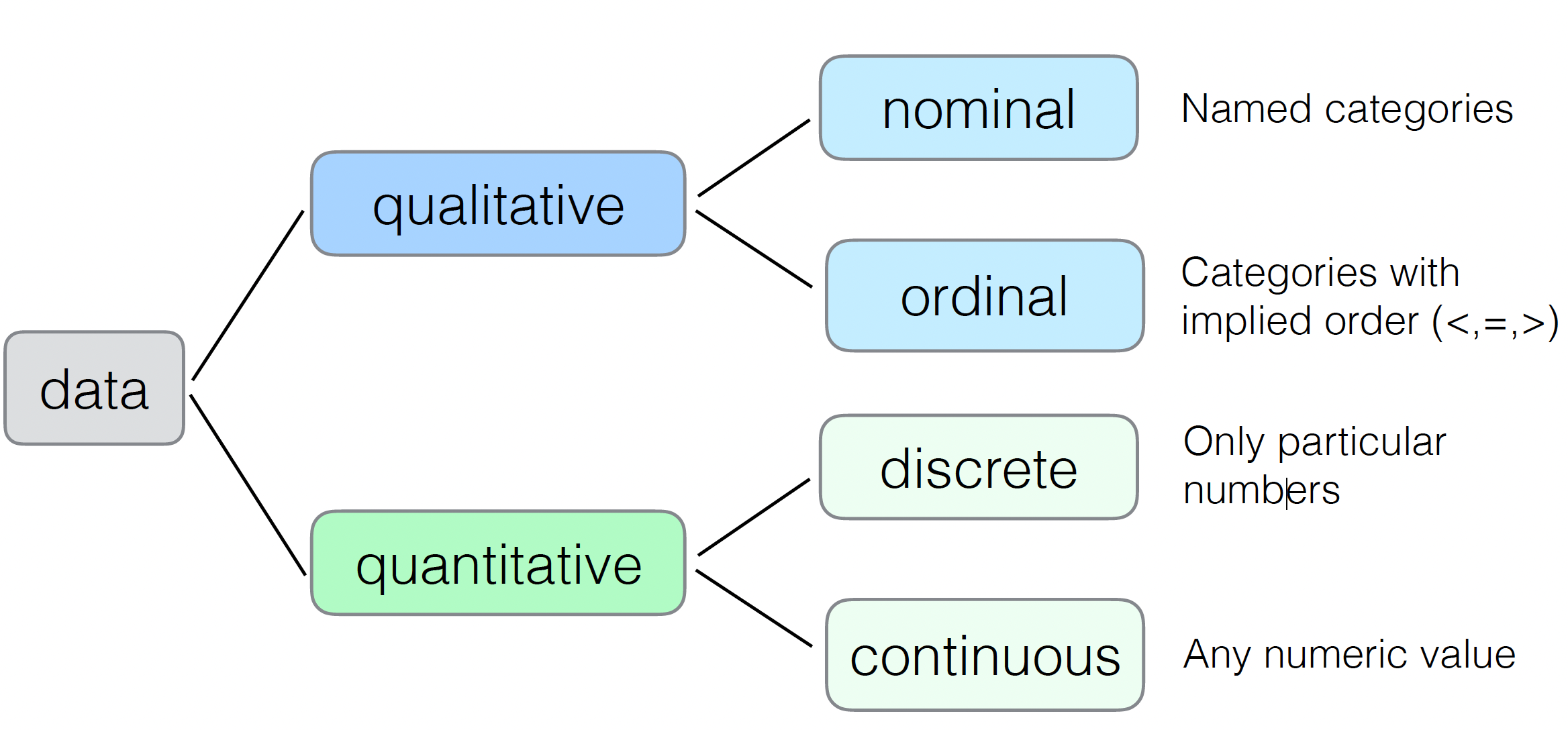
Classify data types
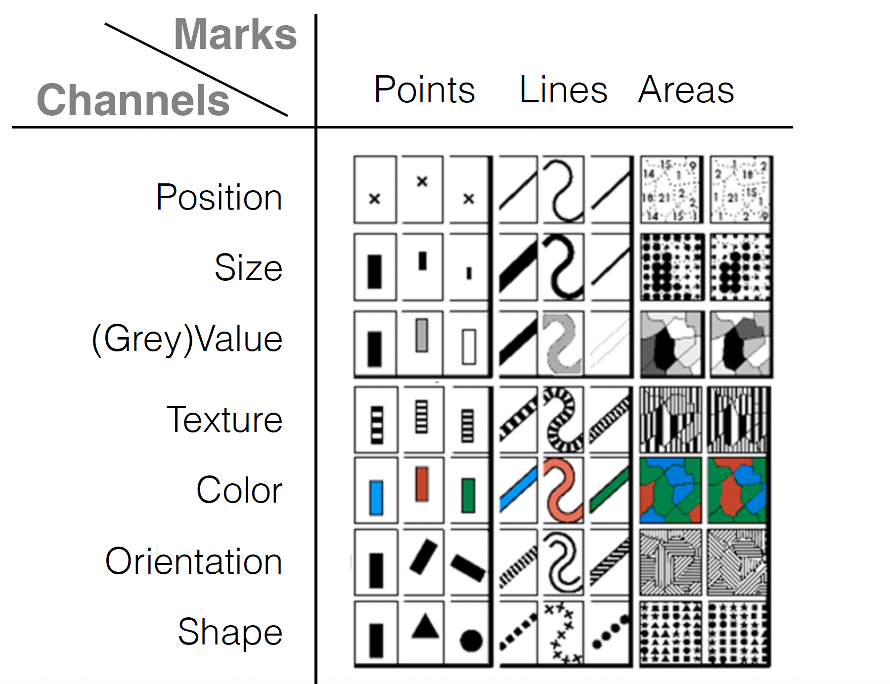
Introducing visual variable
“A visual variable, in data visualization, is an aspect of a graphical object that can visually differentiate it from other objects, and can be controlled during the design process.”
- Jacques Bertin, 1967, Sémiologie Graphique

45 ways to visualizae two quantities
https://rockcontent.com/blog/45-ways-to-communicate-two-quantities/
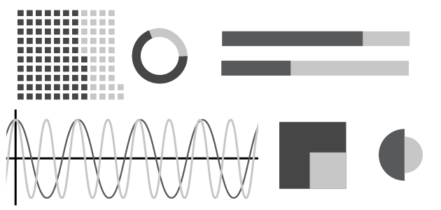
Cleveland’s three visual operations of pattern perception
🎯 Detection: Recognizing that a geometric object encodes a physical value.
🧩 Assembly: Grouping detected graphical elements into patterns.
📏 Estimation: Visually assessing the relative magnitude of two or more values.

What visual cues are most effective for which type of data?
Source: Yau, N. (2013). Data Points: Visualization That Means Something. Wiley.
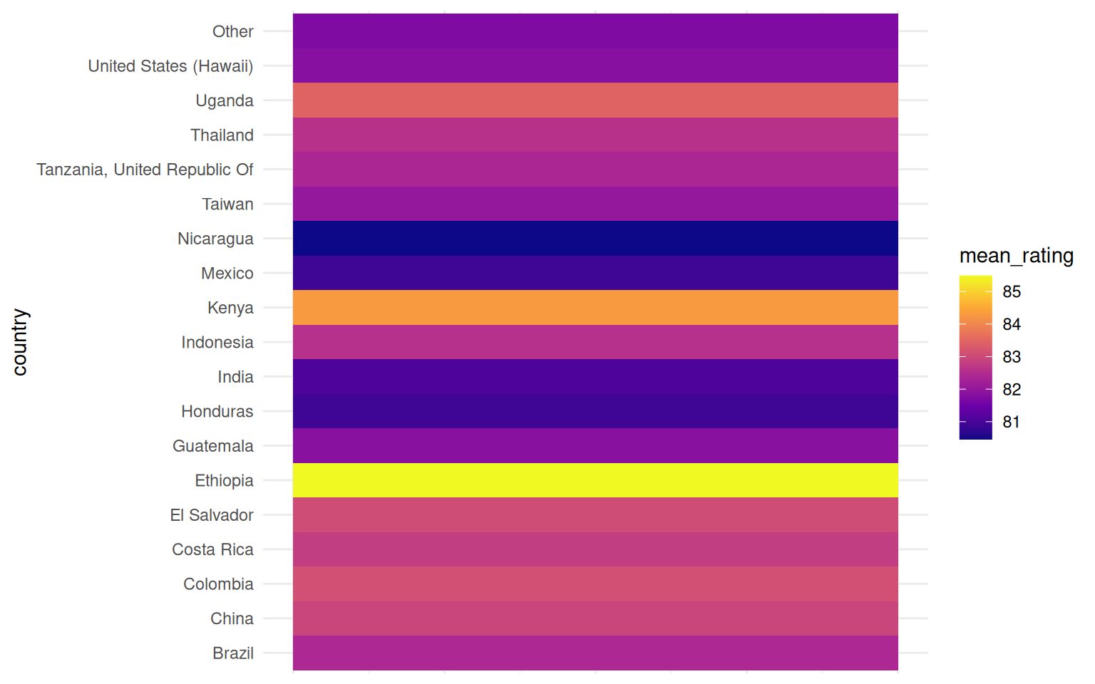
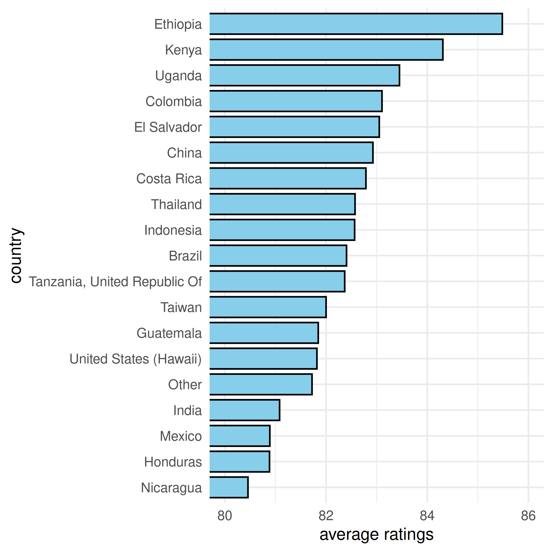
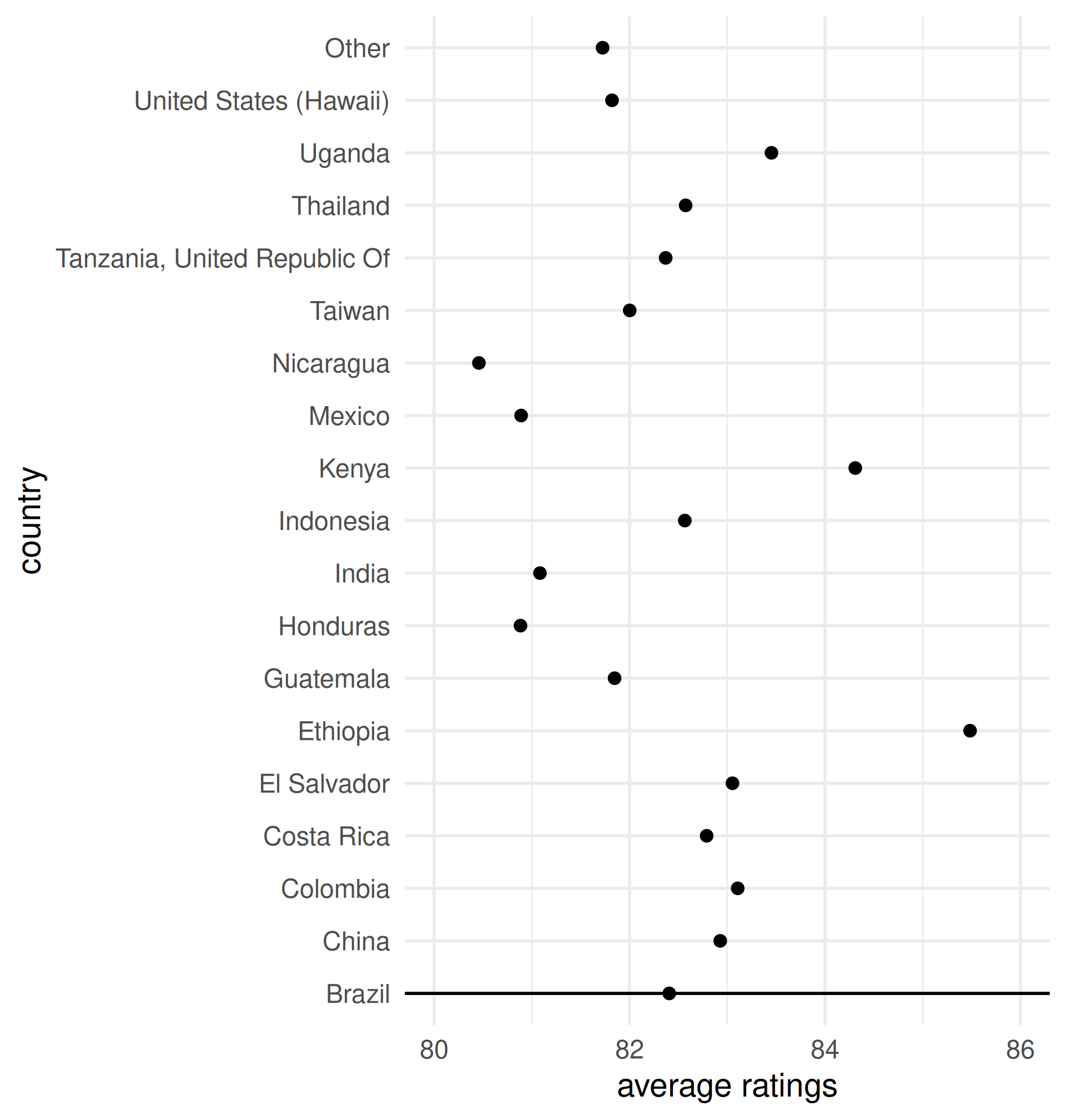
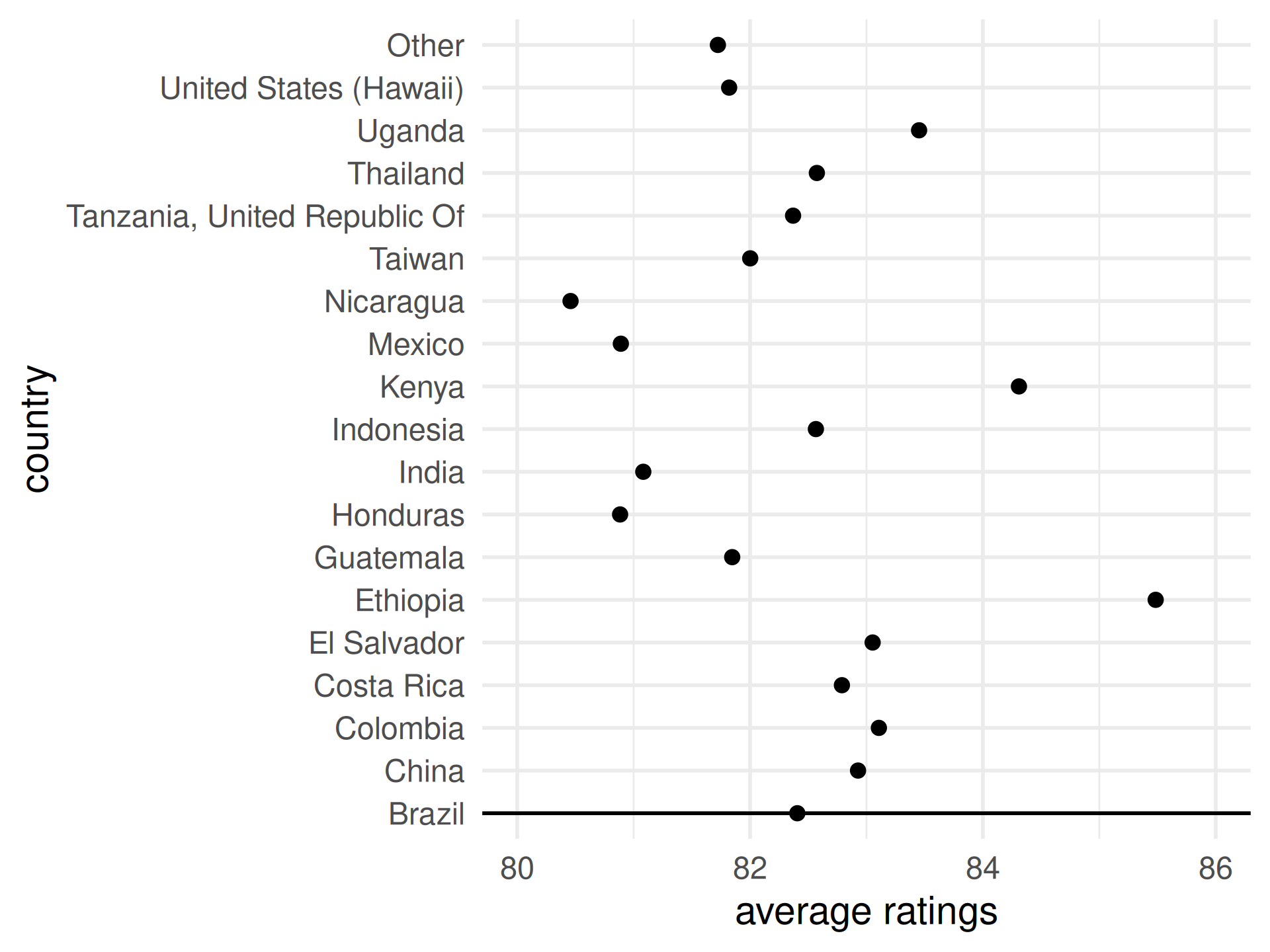
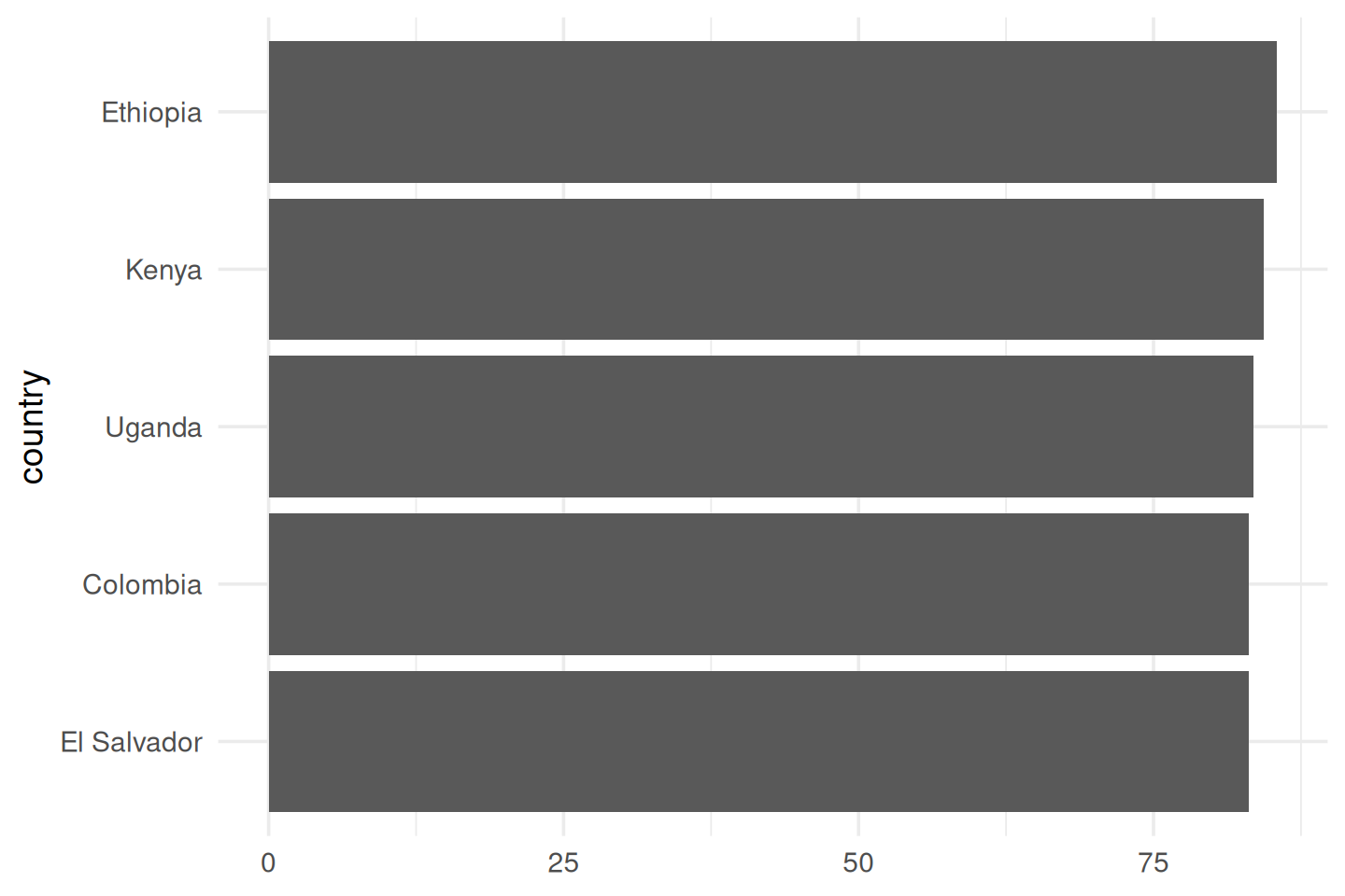
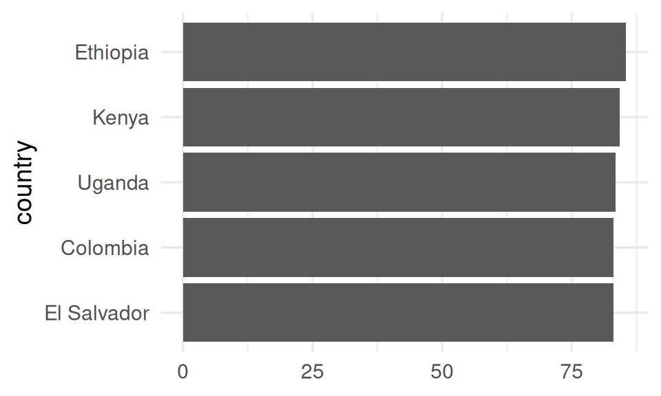
Use color hue to visualize average ratings
Easy: which has higher ratings, Kenya or Indonesia?

Use color hue to visualize average ratings
Hard: which has higher ratings, Indonesia or Costa Rica?
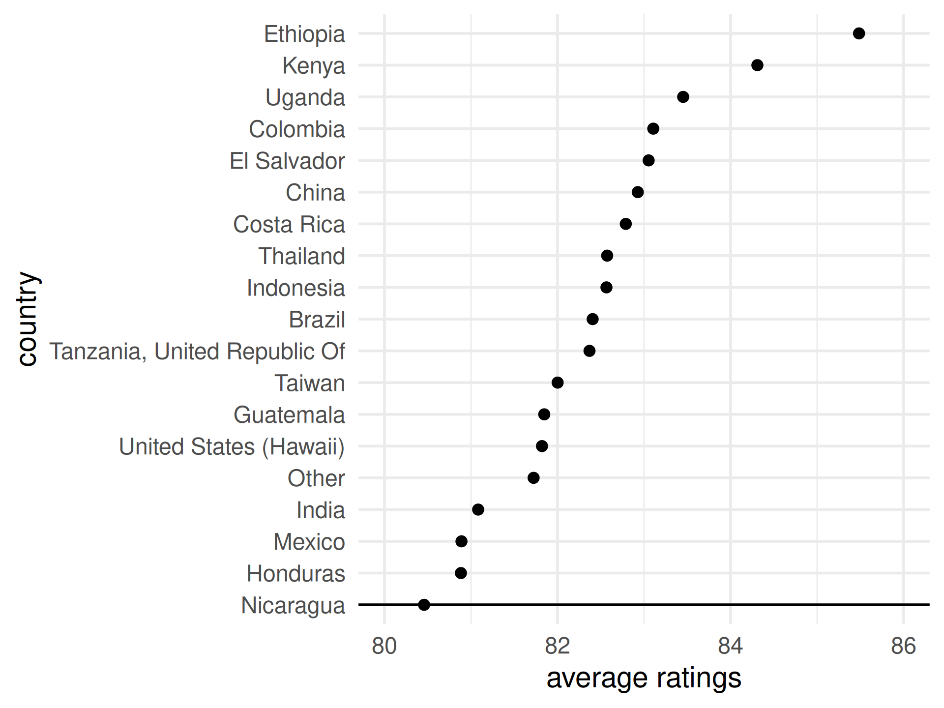
What about now?
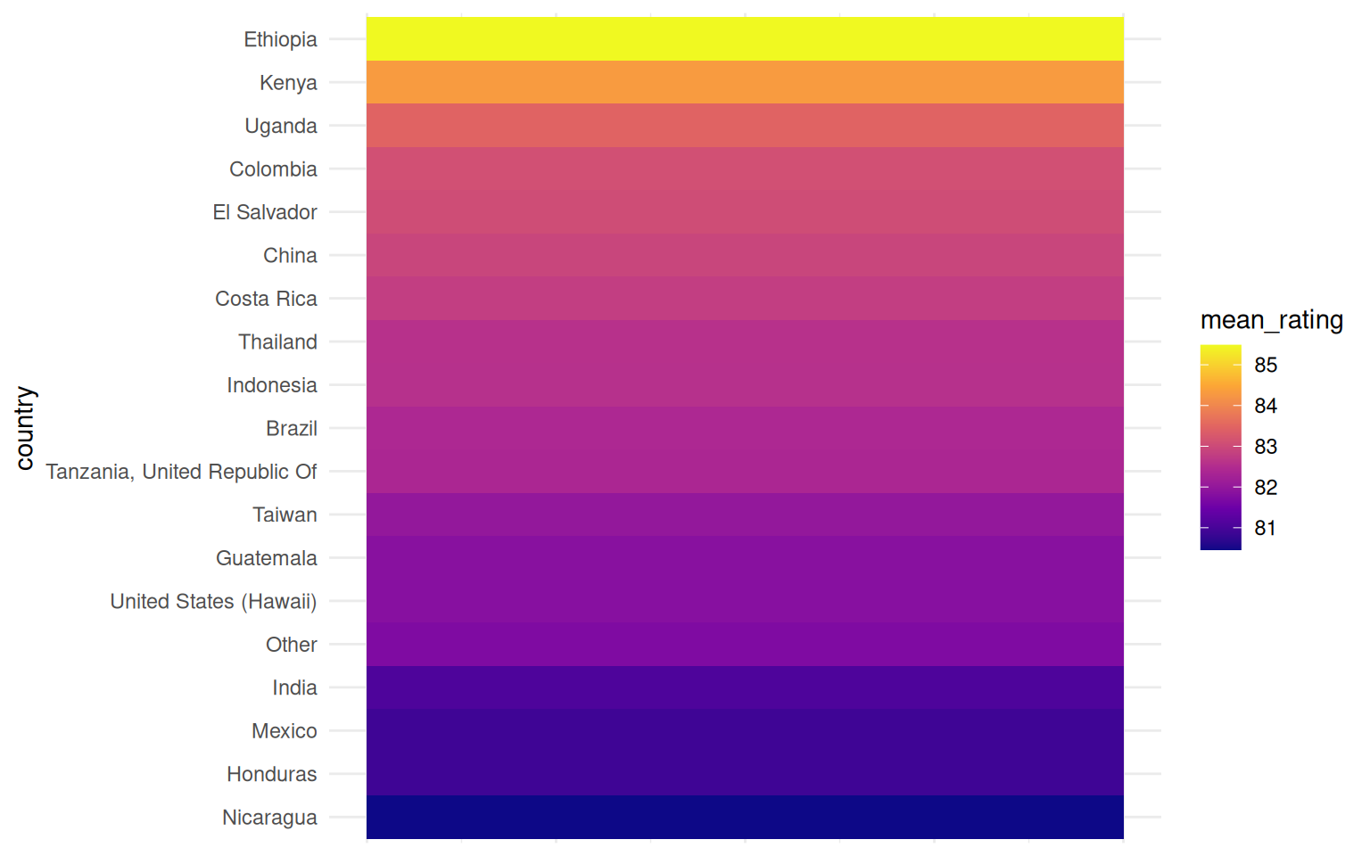
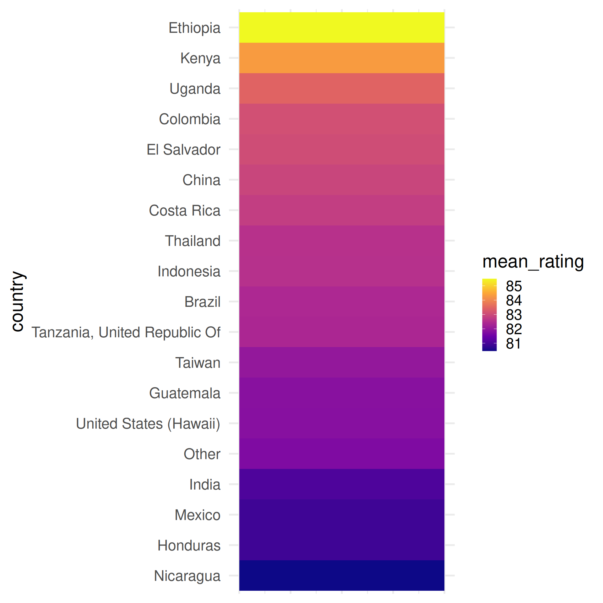
Observation: alphabetical ordering of the categorical variable is almost never useful, re-rank as needed.
Use color saturation to visualize average ratings
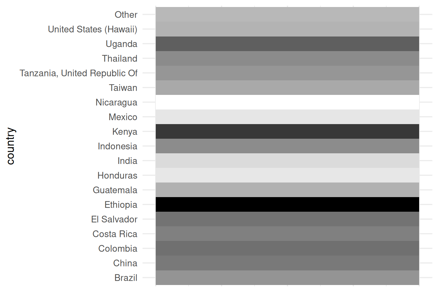
No legend?
No problem.
Because color saturation has natural ordering.
Color saturation is easier to quantify
The ratio between Mexico and United States is…
2 or 3
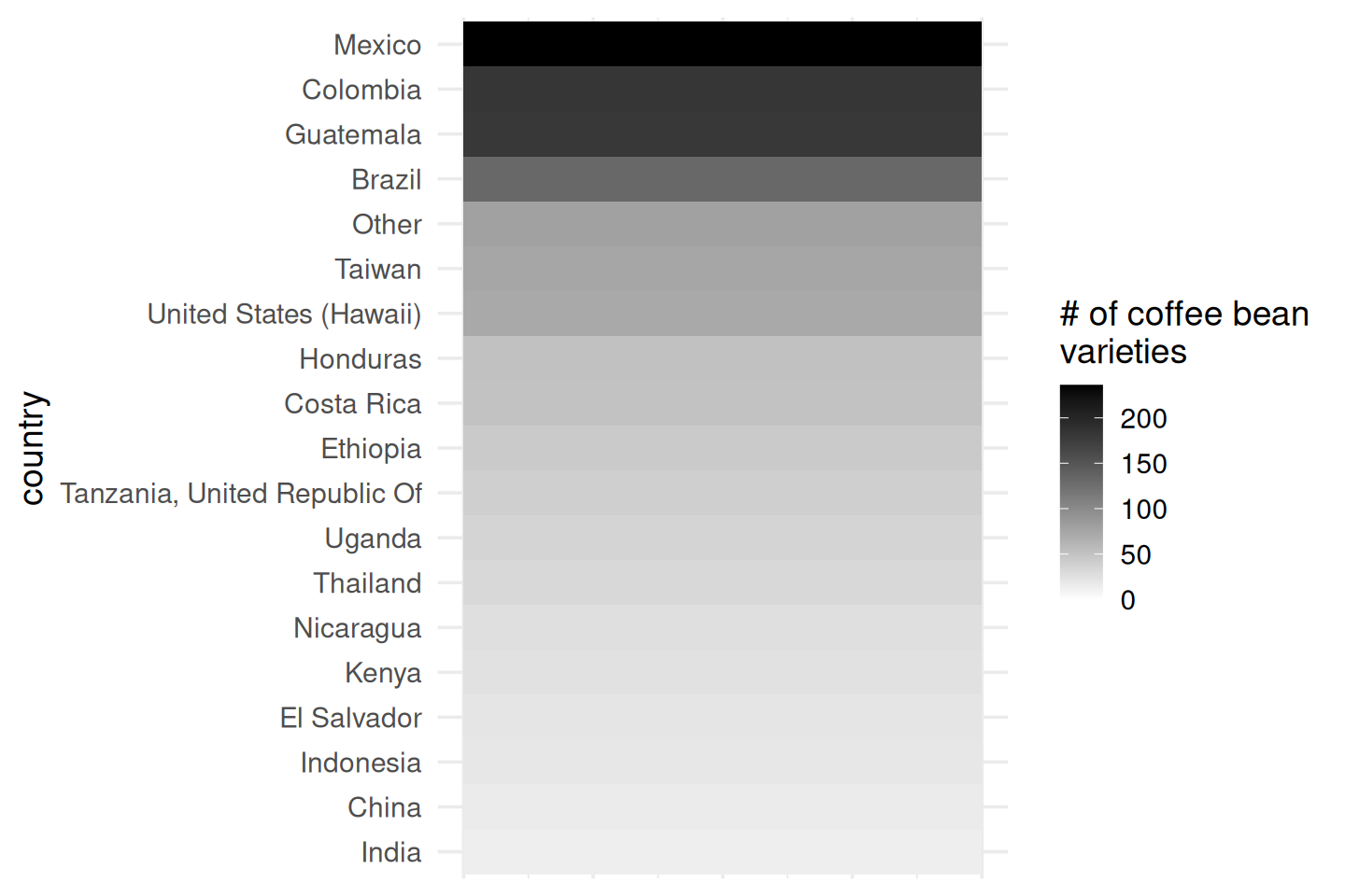
Moving down to the third level of estimation
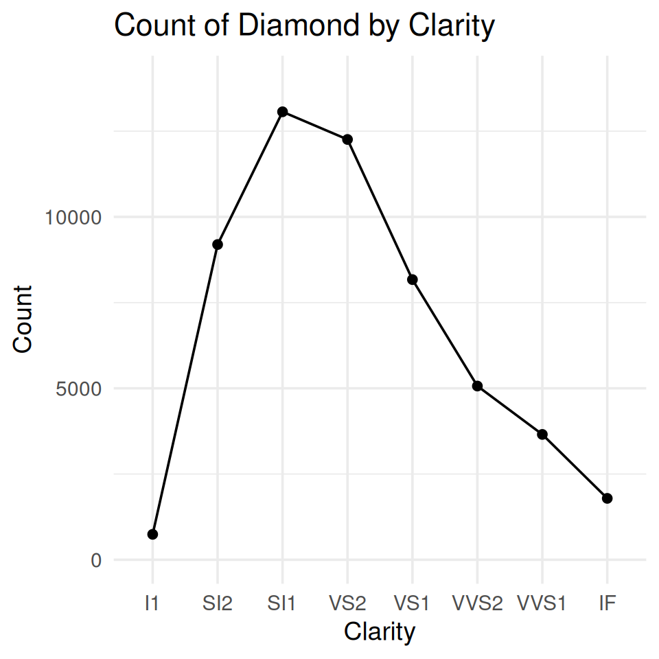
This is weird graph but still informative
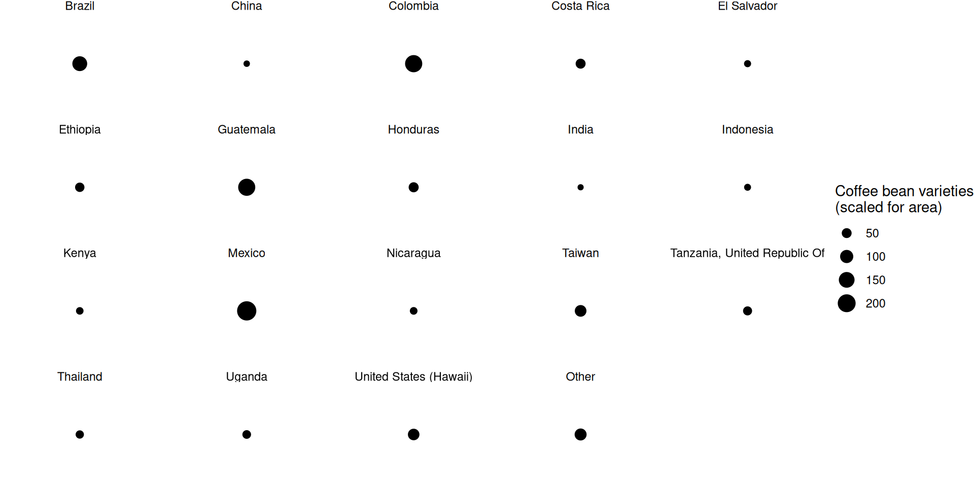
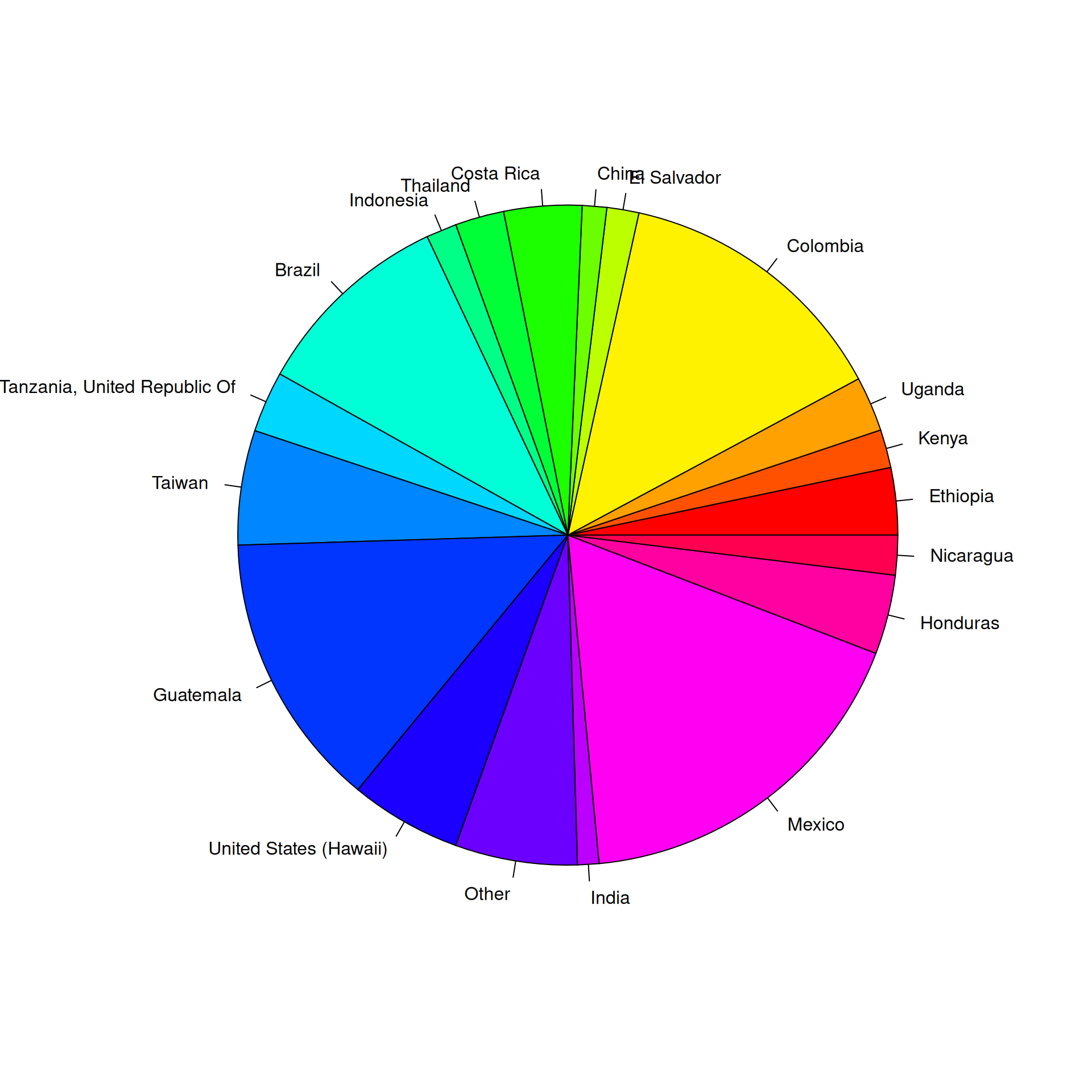
Use angle to visualize coffee bean varieties
Pie charts use angles to encode data
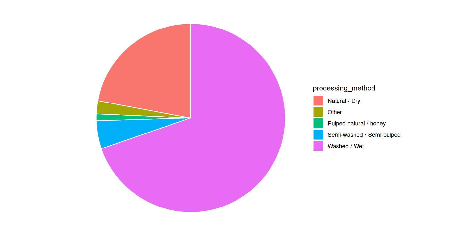
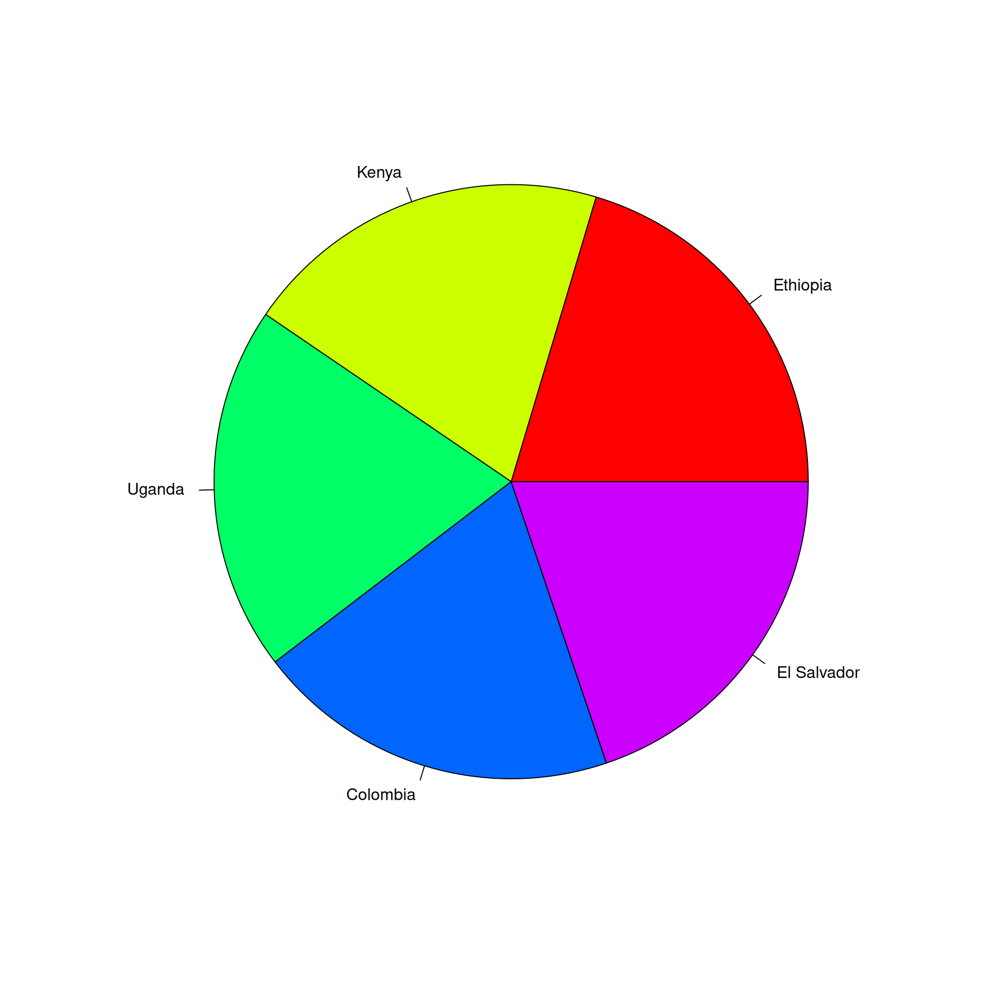
For categorical data, no more than 6 colors is best.
(Source: European Environment Agency)
We are so close!
- Position on a common scale
- Position on non-aligned scales
- Length
- Angle
- Area
- Volume <> Density <> Color saturation
- Color hue

Wait, I thought there is some difference…
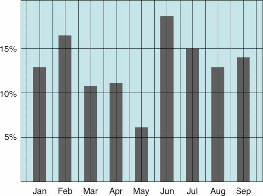
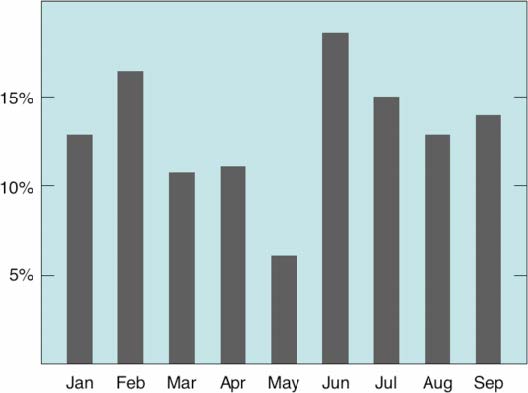
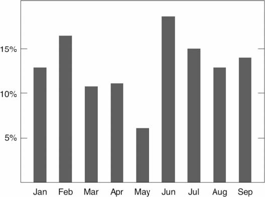
The start-at-zero rule
How to Lie with Statistics (1954)
- Darrell Huff argues that truncating the y-axis can exaggerate differences and mislead the viewer.
- It creates a false impression of dramatic change where the actual variation is small.
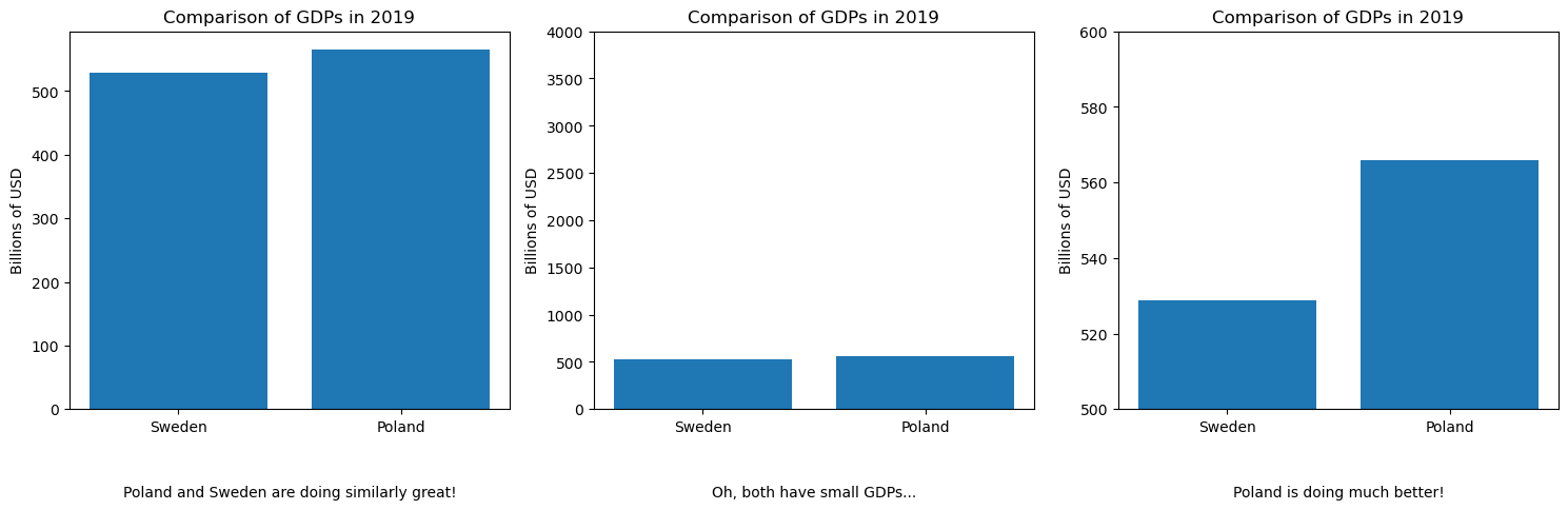
The Visual Display of Quantitative Information (1983)
- Edward Tufte prioritizes data density and the detection of subtle patterns.
- He argues that starting at zero can waste valuable space, obscuring meaningful variations.
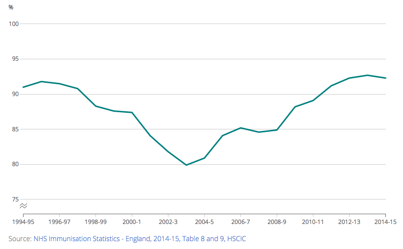
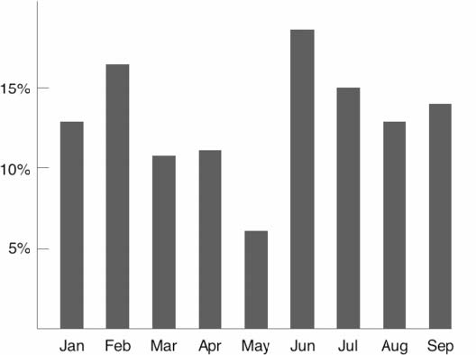
Combined MMR vaccination rate, 1994/95 to 2014/15, England
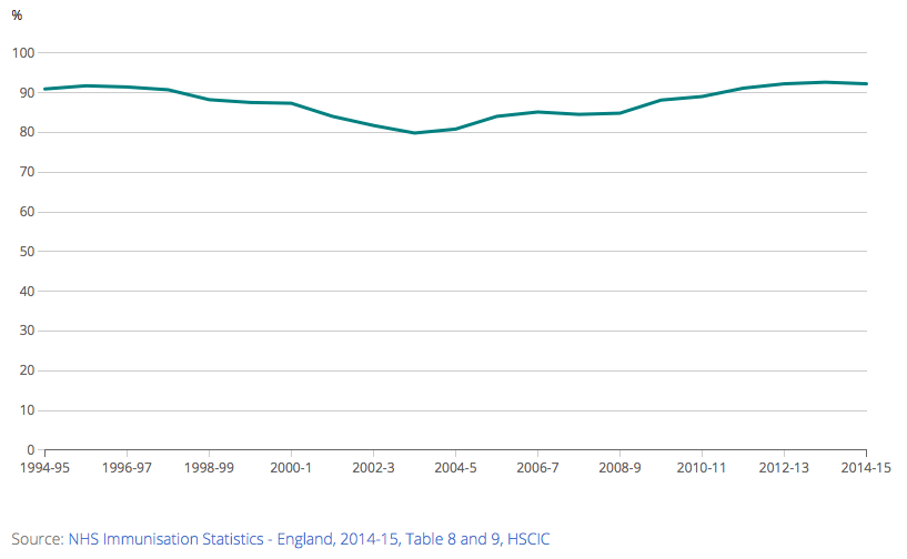
Take another look, axis doesn’t start at zero
Position, but not a common scale
- Position on a common scale
- Position on non-aligned scales
- Length
- Angle
- Area
- Volume <> Density <> Color saturation
- Color hue

Position, and a common scale
- Position on a common scale
- Position on non-aligned scales
- Length
- Angle
- Area
- Volume <> Density <> Color saturation
- Color hue

Position, and a common scale
- Position on a common scale
- Position on non-aligned scales
- Length
- Angle
- Area
- Volume <> Density <> Color saturation
- Color hue
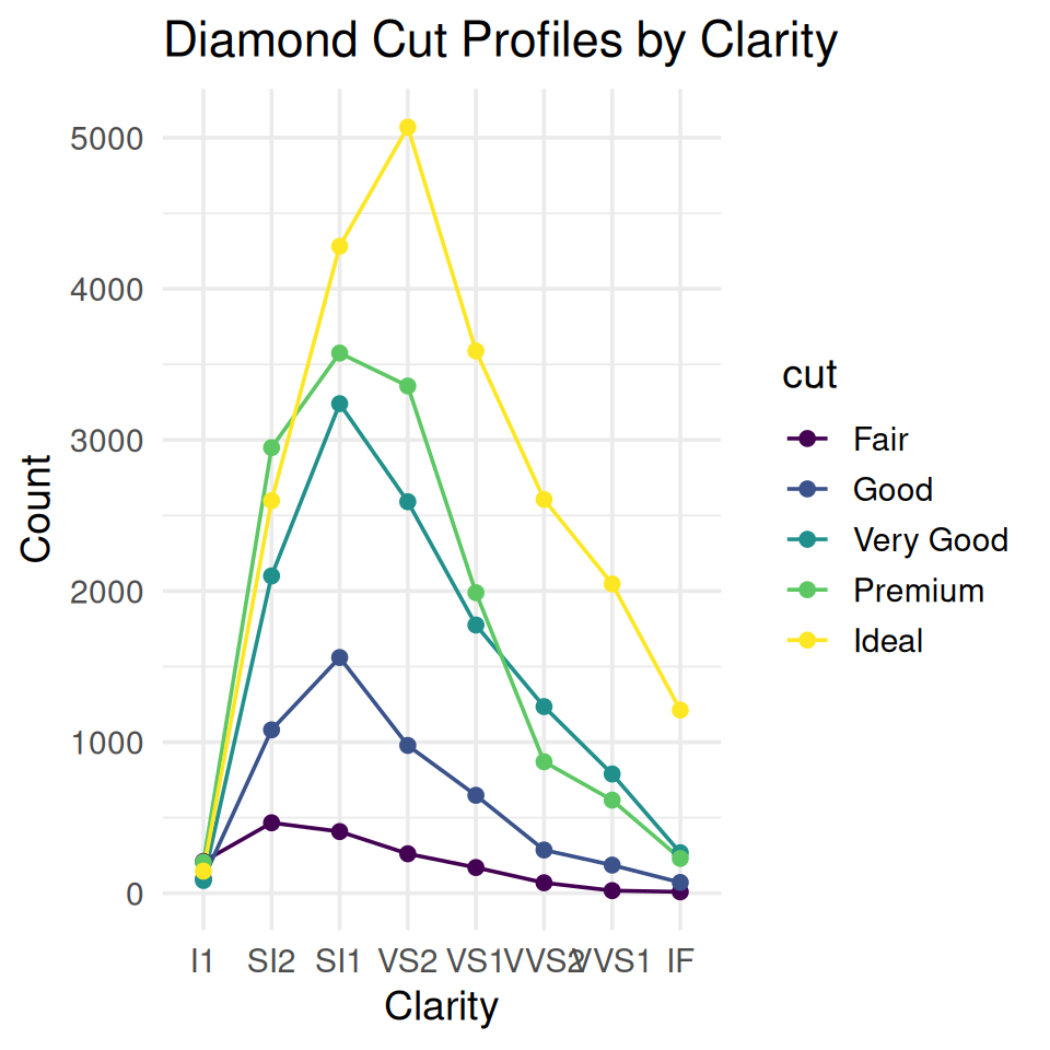
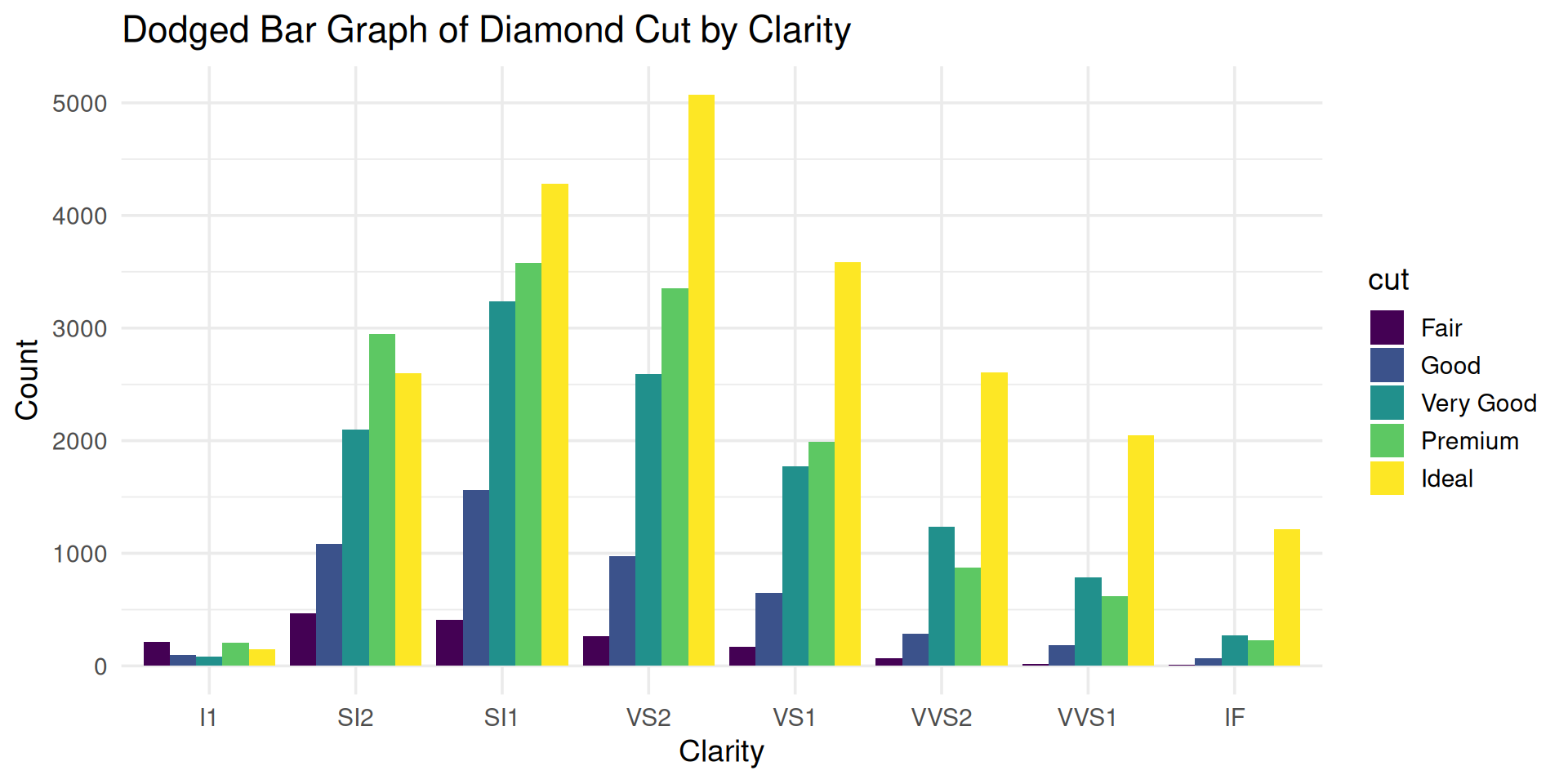
Re-ranking categorical variables still matters!
Stacked anything is nearly always a mistake!
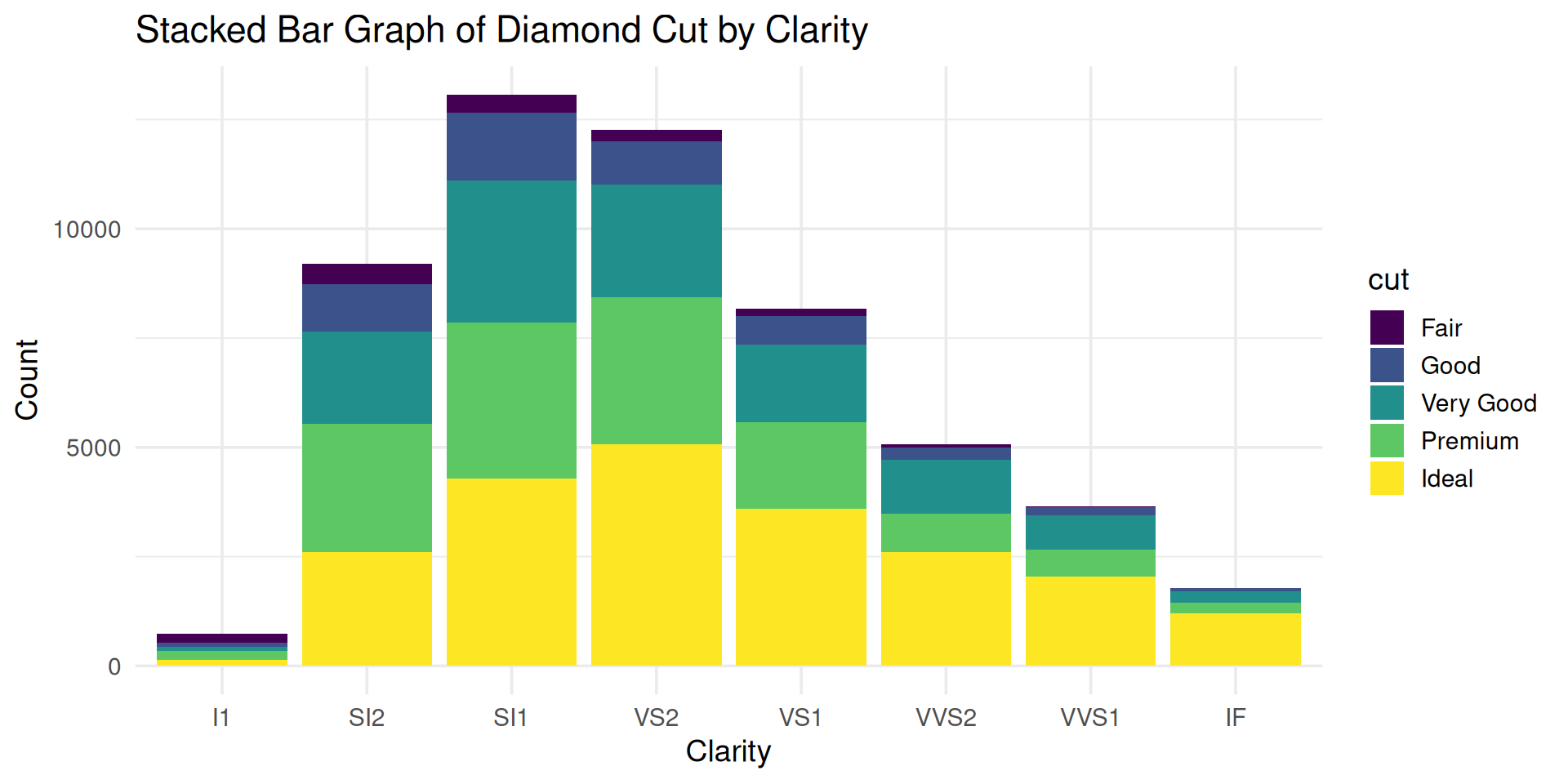
Which category has higher count: SI1-Premium or VS2-Premium?
Transform stacked barplot to a parallel coordinate plot
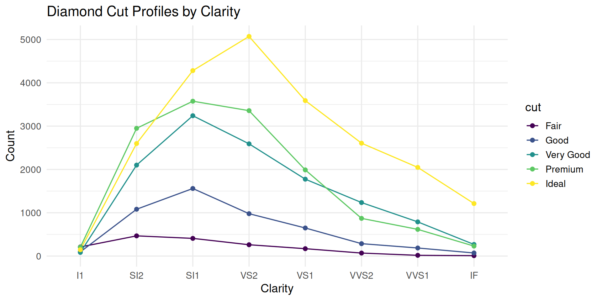
Which category has higher count: SI1-Premium or VS2-Premium?
You lose some information, but just use two charts if needed
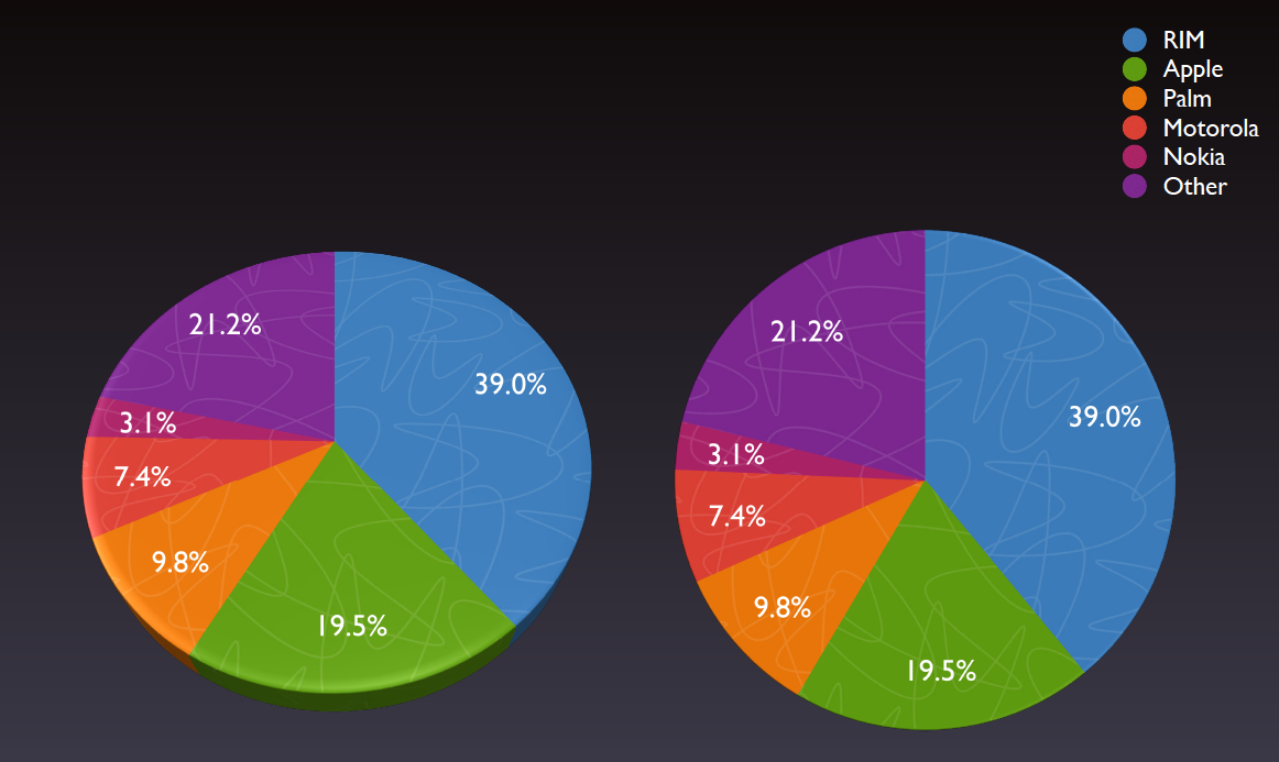
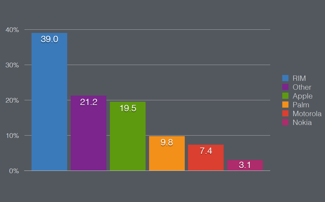
Why are pie charts never a good idea?
Angle is #4 on the accuracy list, we can do better.
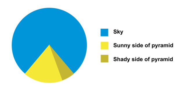
If you have a small amount of data to show, don’t use pie charts
Don’t do this!

Do this instead!
| Label | Value |
|---|---|
| A | 25 |
| B | 60 |
| C | 15 |
If you have a lot of data to show, don’t use pie charts
Don’t do this!
Or this!
All good pie charts are jokes
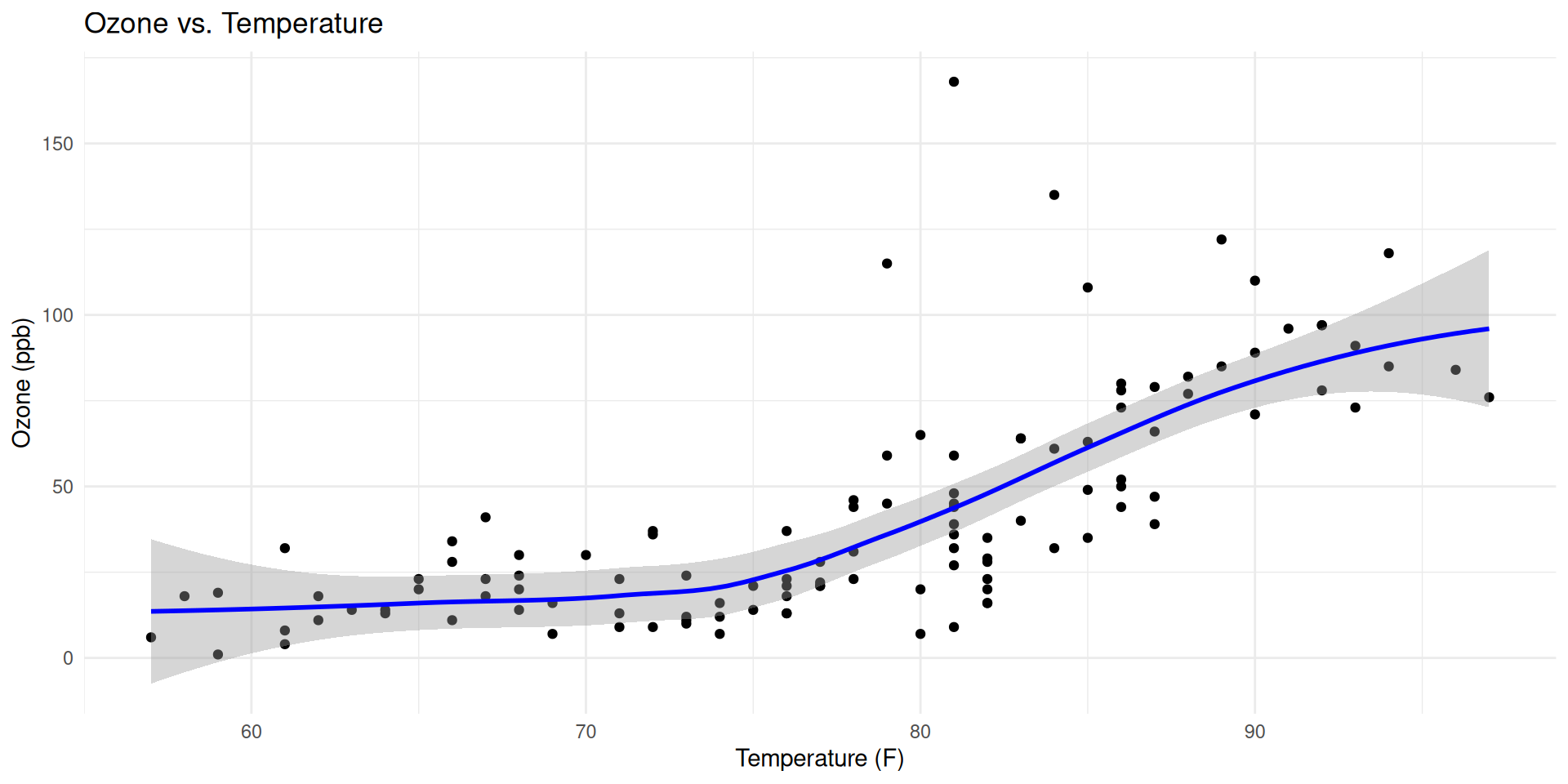
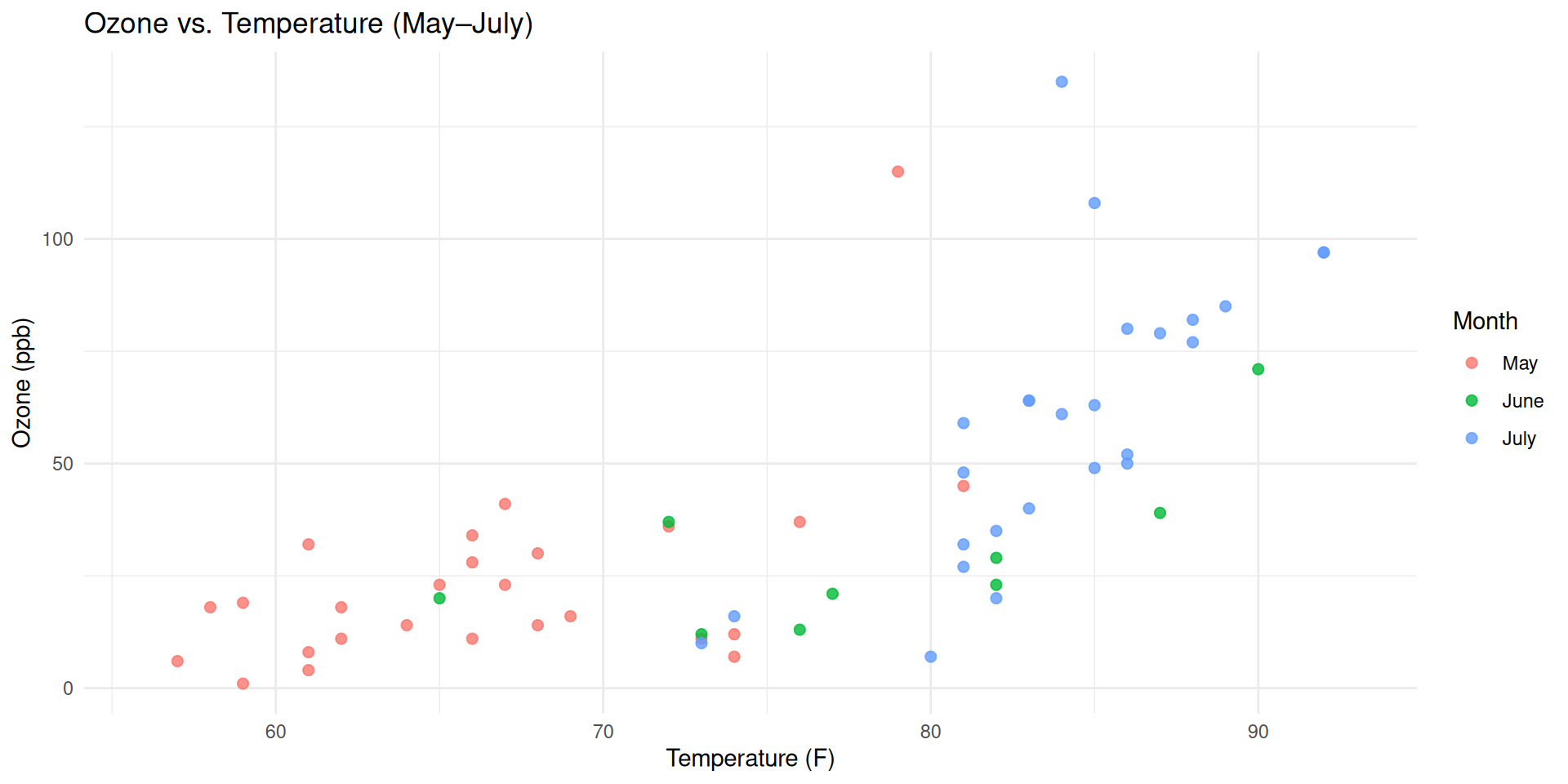
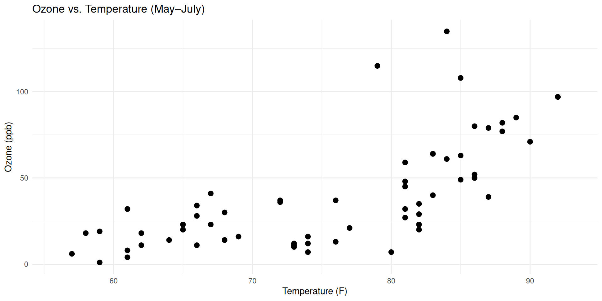
If you want to show the relationship between two variables, use scatterplot
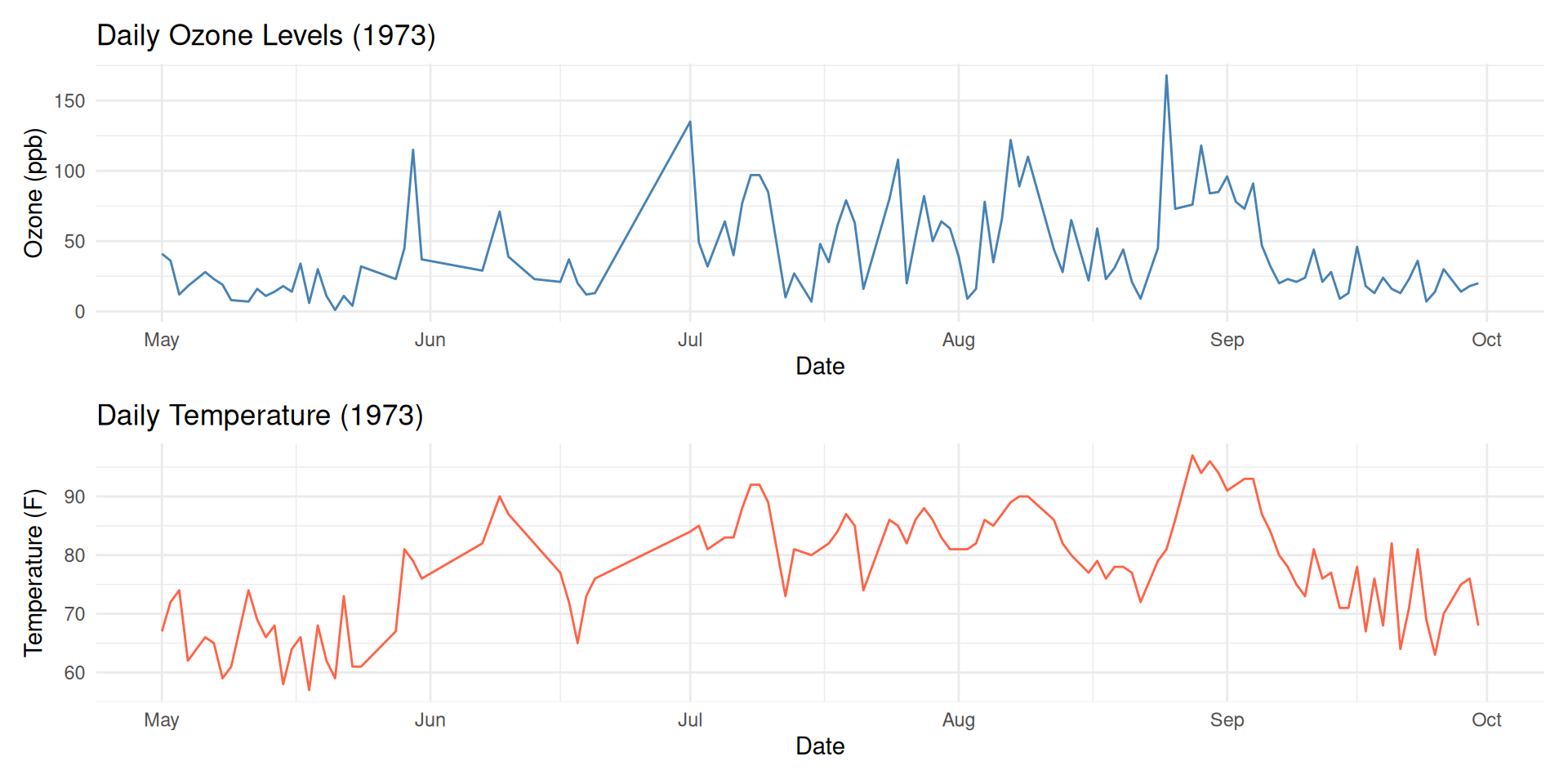
What is the relationship between Ozone concentrations and temperature?
If you want to show the relationship between two variables, use scatterplot
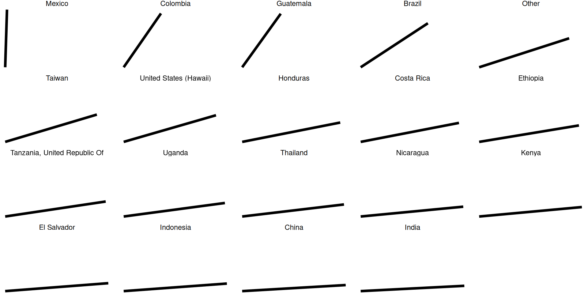
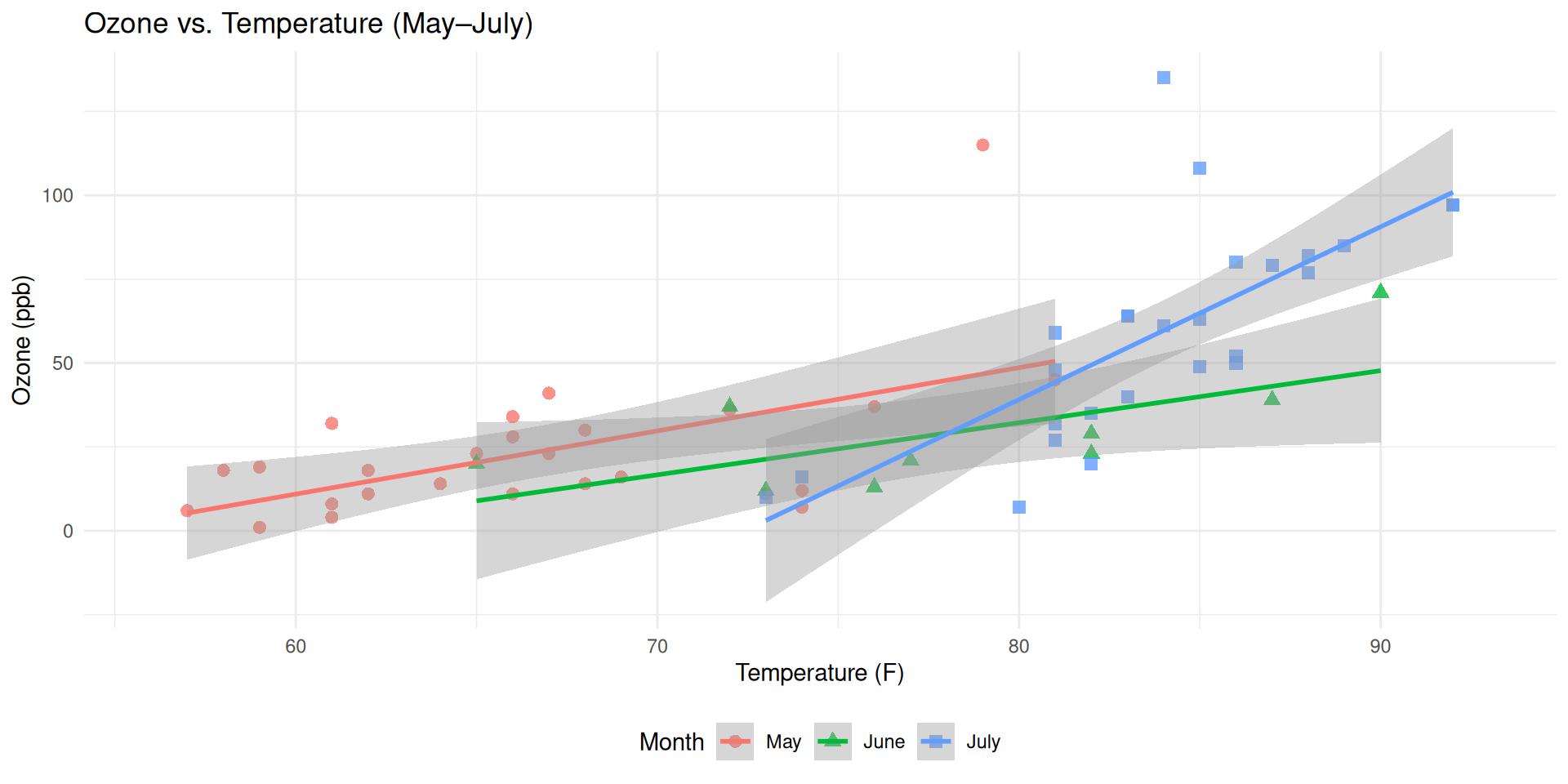
If you care about the growth (slope), plot it directly
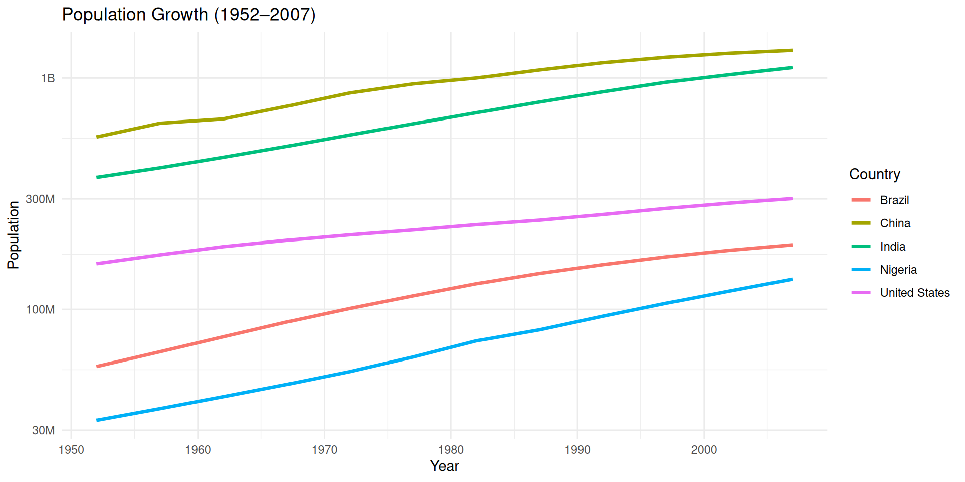
Which country has higher population growth: Nigeria or India?
If you care about the growth (slope), plot it directly
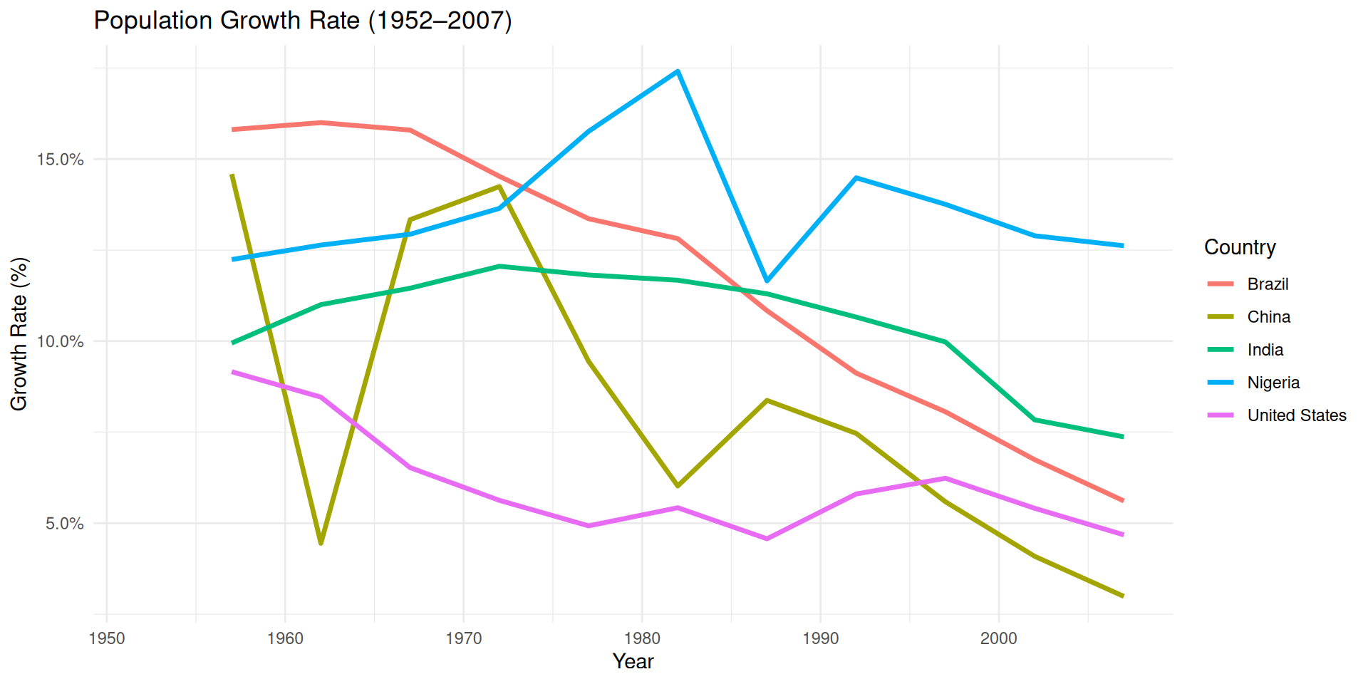
Most countries’ population growth are slowing down, which wasn’t obvious in the previous graph.
Assembly: Gestalt Psychology
“Gestalt (German for form, shape, or configuration). Gestalt psychology proposes that the human brain perceives objects as part of a greater whole rather than as isolated elements.”
Reification

Emergence

Applying Gestalt principles to data visualization
“The law of Prãgnanz, also known as the law of good Gestalt. People tend to experience things as regular, orderly, symmetrical, and simple.”
Law of Continuity 
Law of Similarity
Law of Closure ![]()
Law of Proximity
Bad visualizations lack law of continuity
This hurts our brain.
Good visualizations leverage law of continuity
This is much easier.
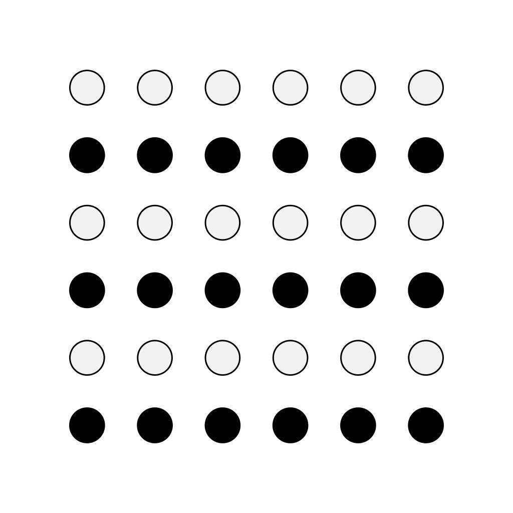
Use law of similarity to group similar data
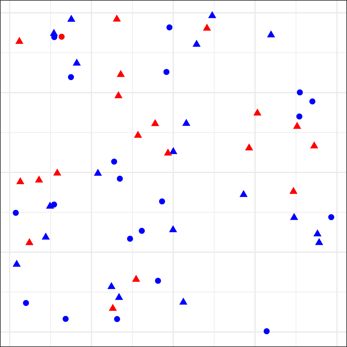
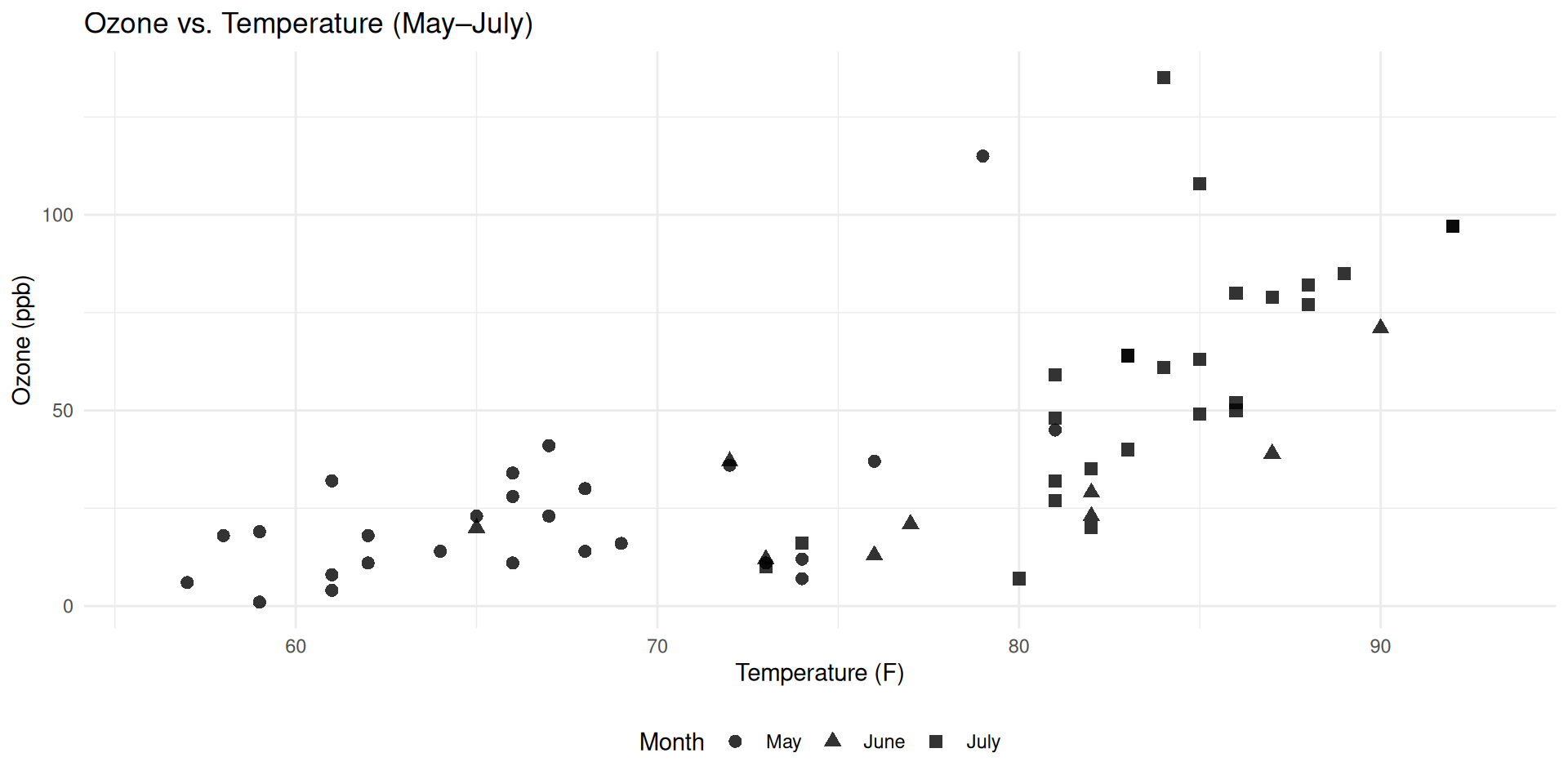
Some encodings are better than others
Shape is less effective than color hue for nominal data
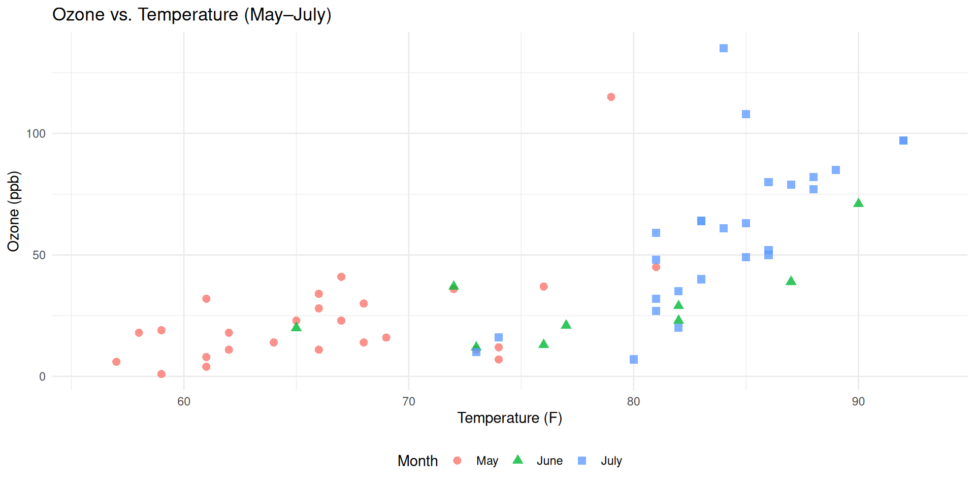
You can combine both color and shape to be more effective
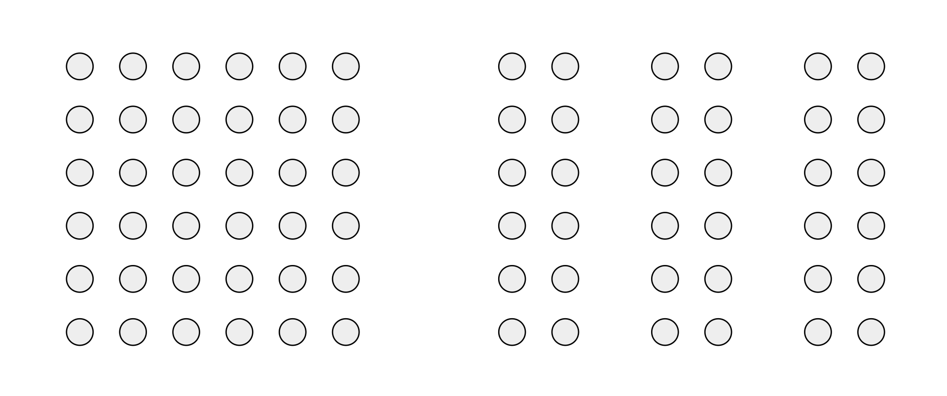
Use law of closure to group similar data
Law of proximity: we see elements near each other as part of the same object
Still worse than parallel coordinate plot

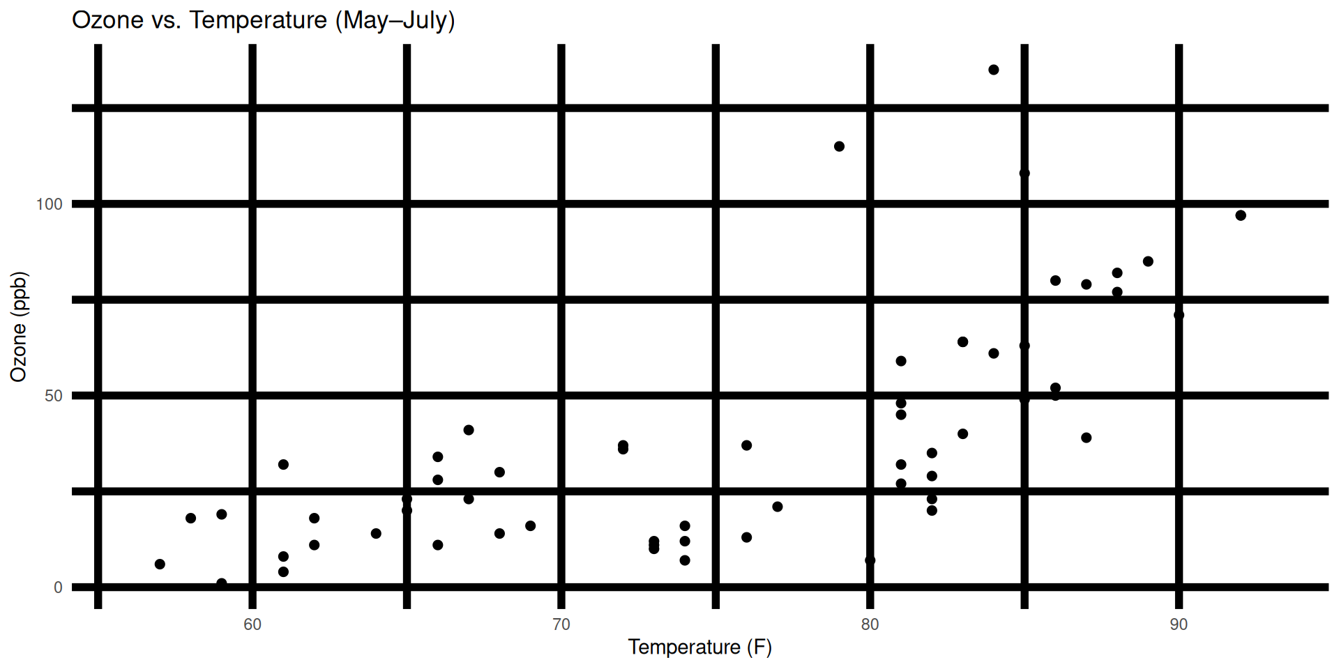
Detection should be trivial, don’t make it hard
Detection should be trivial, don’t make it hard
Detection should be trivial, don’t make it hard
Principles of Graphical Excellence
Graphical excellence is the well-designed presentation of interesting data - a matter of substance, of statistics, and of design.
Graphical excellence consists of complex ideas communicated with clarity, precision, and efficiency.
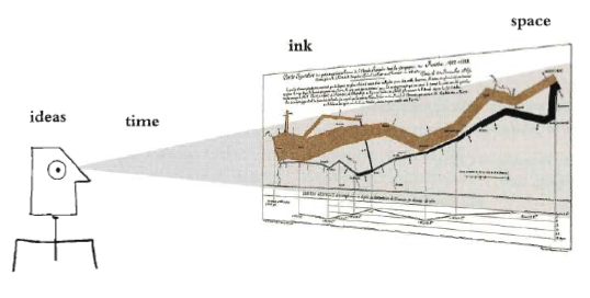
Graphical excellence is that which gives the viewer the greatest number of ideas in the shortest time with the least ink in the smallest space.
Graphical excellence is nearly always multivariate.
Graphical excellence requires telling the truth about the data.
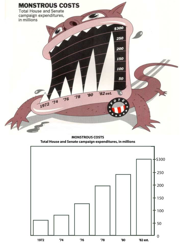
Lie factor
\[ \text{Lie Factor} = \frac{\text{size of effect shown in graphic}}{\text{size of effect in data}} \]
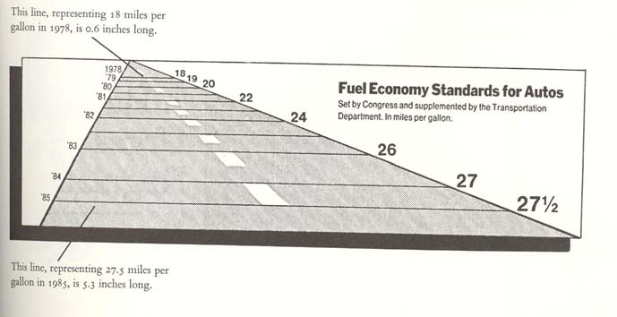
Can you calculate the lie factor in this graph?
Why are 3D graphs bad?
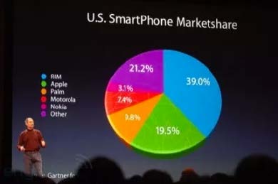
Source: the Guardian, 2008
How should the data be plotted?
Or even better
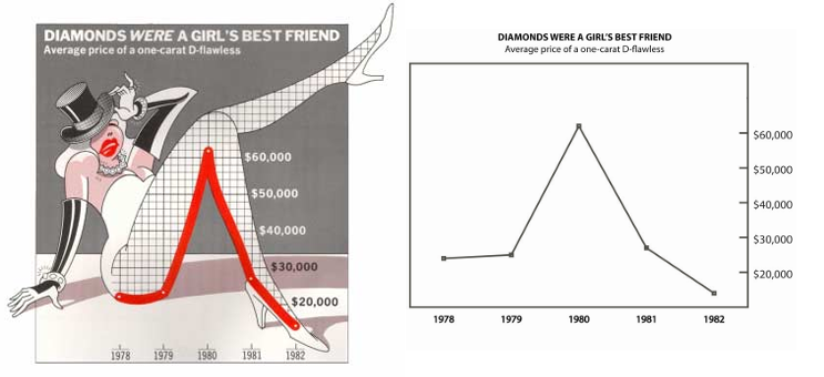
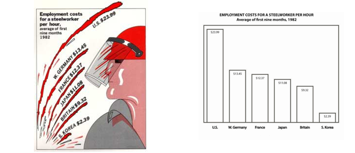
Avoid junk chart
Avoid junk chart
Avoid junk chart
Avoid junk chart
Avoid junk chart

Avoid junk chart

Data density in graphical practice
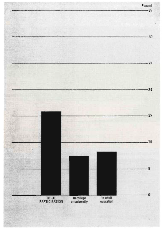
Office of Management and Budget
Social Indicators, 1973
\[ \text{data density of a graphic} = \frac{\text{number of entries in data matrix}}{\text{area of data graphic}} \]
\[ \begin{aligned} \text{data density} &= \frac{\text{2 data points}}{\text{graph covres 26.5 square inch}} \\ &= 0.15 \text{ numbers per square inch} \end{aligned} \]
Data density in graphical practice
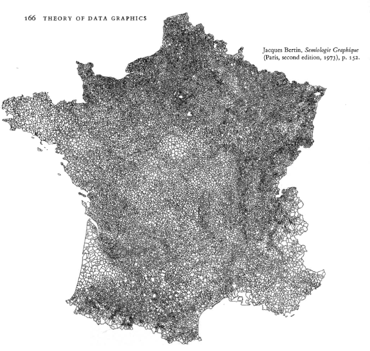
Jacques Bertin, Semiologie Graphique, 1973
\[ \text{data density of a graphic} = \frac{\text{number of entries in data matrix}}{\text{area of data graphic}} \]
\[ \begin{aligned} \text{data density} &= \frac{\text{240,000 data points}}{\text{graph covres 27 square inch}} \\ &= 9,000 \text{ numbers per square inch} \end{aligned} \]
How to create high-information graphics design?
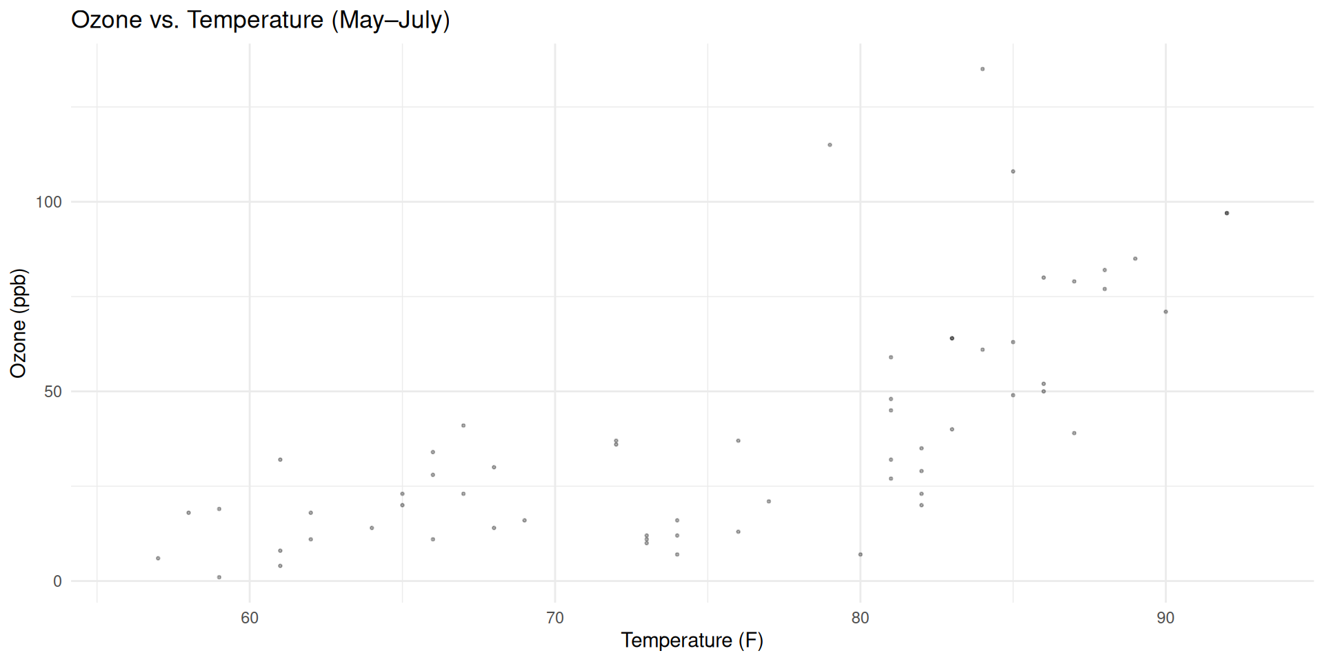
Graphics can be shrunk way down
Default size
Appropriate size
Small Multiples
“Small multiples resemble the frames of a movie: a series of graphics, showing the same combination of variables, indexed by changes in another variable.”
Tufte, E. R. (1983). The Visual Display of Quantitative Information. Cheshire, CT: Graphics Press.
Tufte’s design principles
- Graphical integrity
- The Lie Factor
- Maximize data-ink ratio
- Avoid chart junk

Most useful for analytical or technical audience, e.g. scientists, engineers, and data analysts. Less useful for the general public or media campaigns.
Useful junk