Lecture 4.Introduction to R Shiny

PUBH 6199: Visualizing Data with R, Summer 2025

Xindi (Cindy) Hu, ScD

2025-06-10

Outline for today

What is R Shiny
Write a basic R shiny app
Deploy your Shiny apps with shinyapps.io
AI-powered help: using Shiny Assistant

About R Shiny

Shiny is an R package that makes it easy to build interactive web applications (apps) straight from R
Shiny allows users to build dynamic, data-driven web apps without requiring extensive knowledge of web development
To install R Shiny run the following command in the console of your RStudio install.packages("shiny")

Key Features

Interactive Web Applications: Shiny makes web apps that respond to user inputs
Seamless Integration with R: Users can leverage the full power of R, like data manipulation, statistical modeling, and plotting
Easy Deployment using Shiny Cloud
Extensibility: Shiny apps can be enhanced with custom HTML, CSS, and JavaScript

Basic Structure Shiny Application

A typical Shiny application has two main components:
- User Interface (UI): Defines the layout and appearance of the app, including input controls (like sliders and text boxes) and output displays (like plots and tables).
- Server Function: Contains the logic that processes inputs and generates outputs. It reacts to user interactions

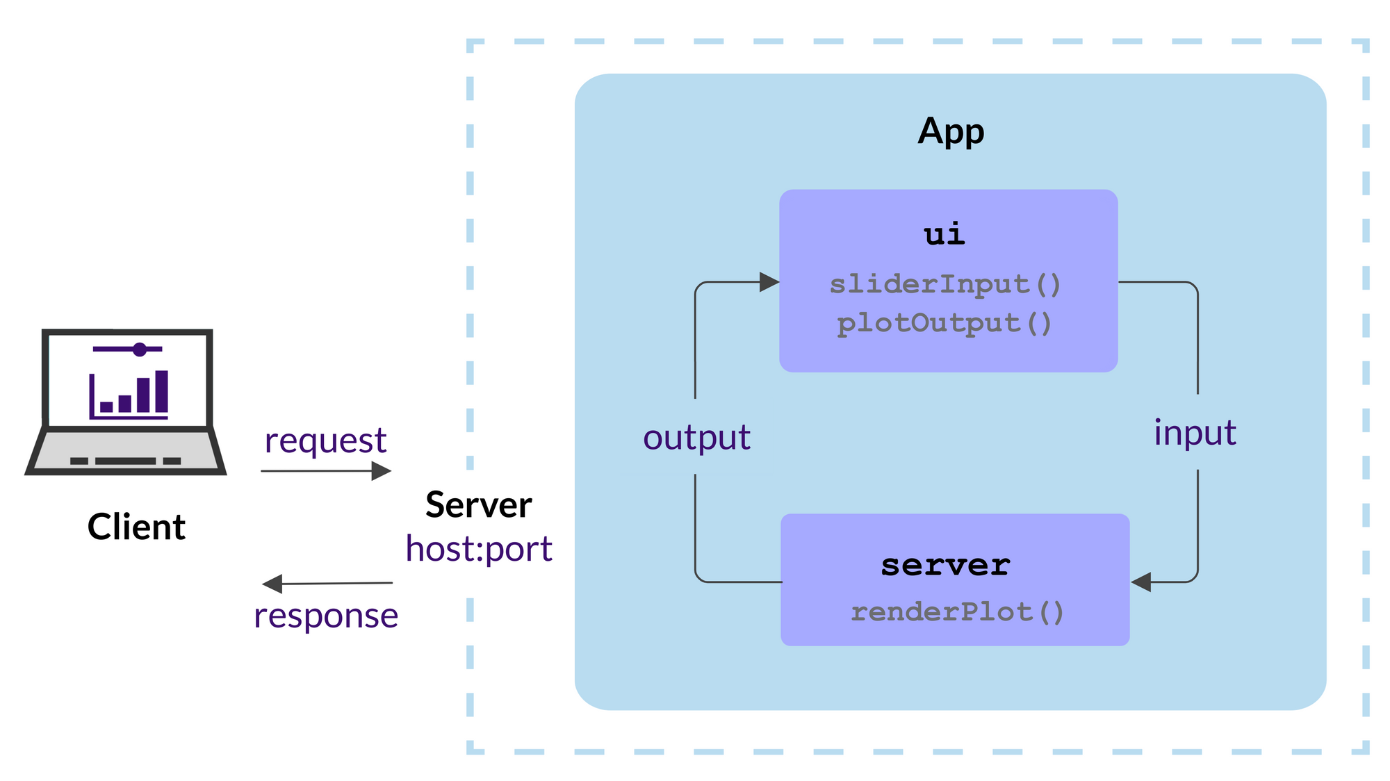
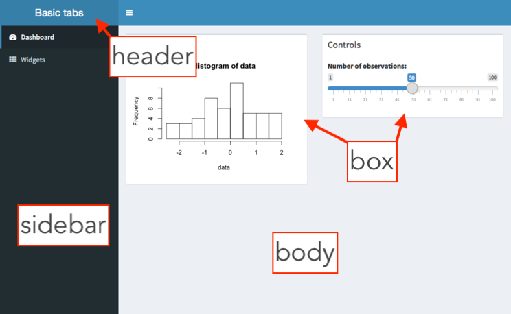
Visual Logic

Here we can see the visual logic behind a Shiny application

`Input()`, `Output()` and `render*()`

These three groups of functions are the core of Shiny’s reactive programming model:

*Input(): Represents user inputs, such as text input, slider input, or checkbox input. For example, input$sliderValue retrieves the value of a slider input with the ID “sliderValue”.
*Output(): Represents outputs that are displayed in the UI, such as plots, tables, or text. For example, output$histPlot refers to a plot output with the ID “histPlot”.
render*(): Functions that generate outputs based on inputs. For example, renderPlot() creates a plot output, and renderText() generates text output. These functions are reactive and will automatically update when the inputs change.

`*Input()` function syntax

Shiny input functions: sliderInput(), selectInput(), textInput() numericInput(), etc.

General format:

inputFunction(inputId, label, value, ...)

inputId: connects UI and server via input$inputId, must be a simple string without spaces, must be unique within the app
label: text label for the input control, displayed in the UI
value: initial value of the input control, can be a number, character, or logical value. For example:

# use position for inputId and label
# use named args for the rest
sliderInput("min", "Limit (minimum)", value = 50, min = 0, max = 100)

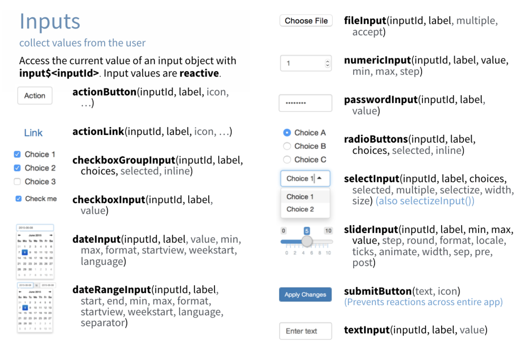
Different types of UI Inputs

Source: Shiny for R cheatsheet

`*Output()` function syntax

Shiny output functions: plotOutput(), tableOutput(), textOutput(), etc.

What *Output() function does:

Output functions in the UI create placeholders.
These placeholders are filled by the server using a matching render*() function.

General format:

outputFunction(outputId)

outputId: connects UI and server via output$outputId, must be a simple string without spaces, must be unique within the app. For example:

plotOutput("scatterplot")

Accessed in server as:

output$outputId <- renderFunction({...})

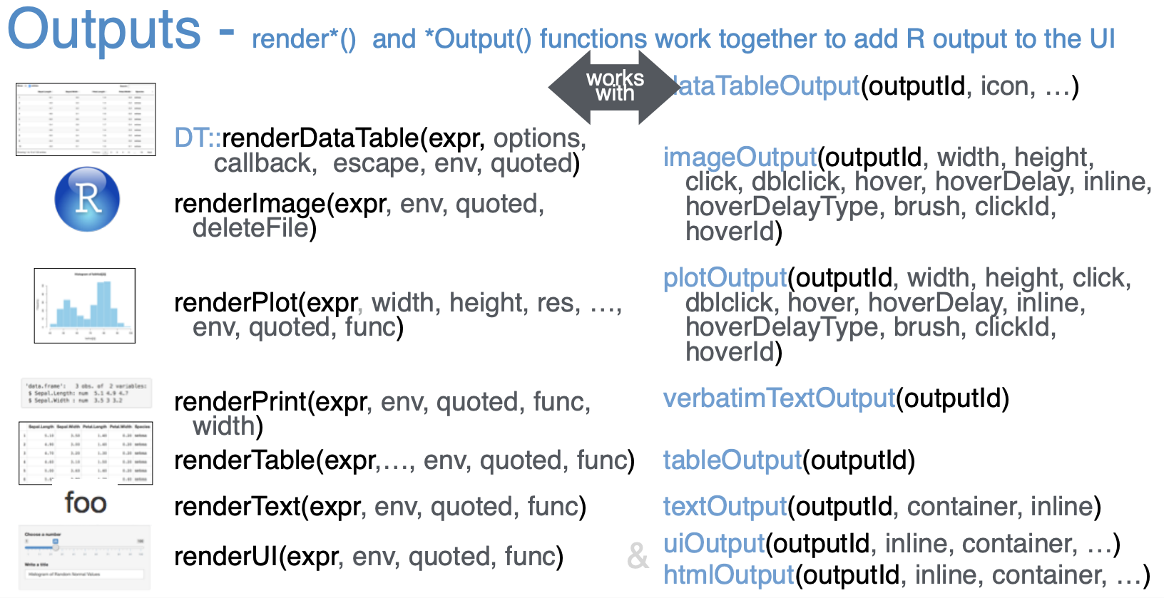
Output <-> Render pairing

# UI
plotOutput("my_plot")
# Server
output$my_plot <- renderPlot({
  ggplot(data, aes(...)) + geom_point()
})

Source: Shiny for R cheatsheet

Outline for today

What is R Shiny
Write a basic R shiny app
Deploy your Shiny apps with shinyapps.io
AI-powered help: using Shiny Assistant

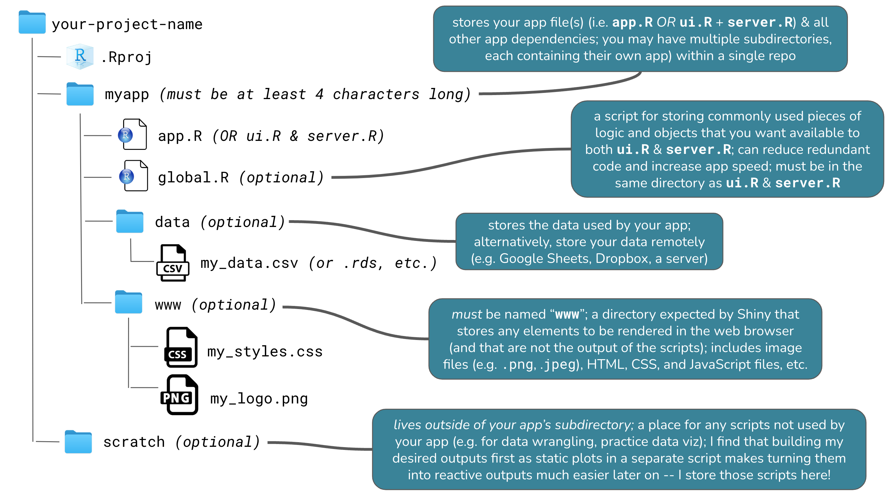
Setting up a shiny app

Create a GitHub repo and clone the repo to our computer
Install R Shiny in your R environment : install.packages("shiny")
Organize repo structure

Two options for shiny apps

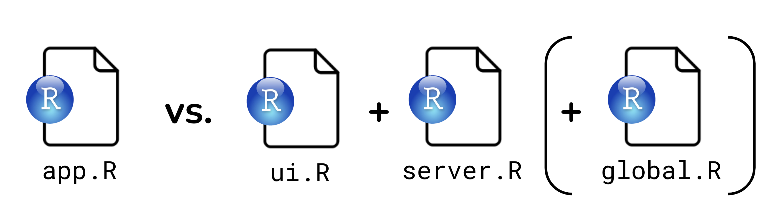
Single-File App: All code is in one file, typically named app.R. This is suitable for simple applications or creating a reprex example.

Two-File App: Code is split into multiple files, usually ui.R for the user interface and server.R for the server logic. Optionally, global.R can be used for data ingestion and wrangling. This is better for larger applications.

Create a single-file Shiny app

Create a new R script file named app.R
The file should contain both the UI and server components
The basic structure of a single-file Shiny app is as follows:

# load packages ----
library(shiny)

# user interface ----
ui <- fluidPage()

# server instructions ----
server <- function(input, output) {}

# combine UI & server into an app ----
shinyApp(ui = ui, server = server)

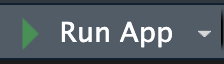
Once you have this structure, RStudio recognize this is a R shiny app and you can run the app by clicking the “Run App” button in RStudio.

Let’s build the app step-by-step

We will create a simple Shiny app that displays a histogram of random normal data
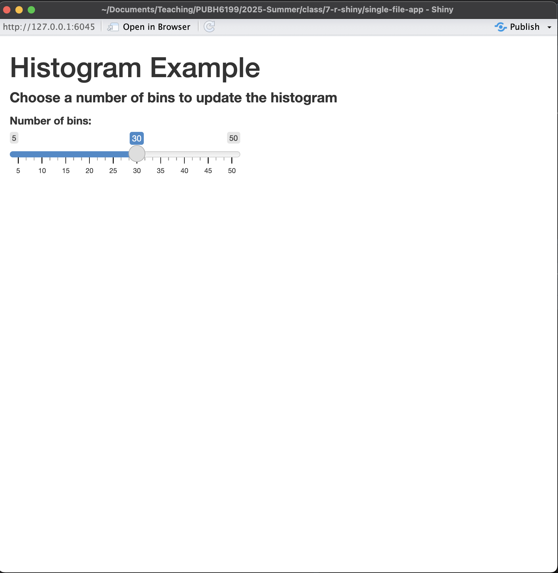
The app has a title and subtitle
Users can adjust the number of bins in the histogram using a slider input
The histogram will react to the slider input and update accordingly

Code Breakdown UI

Calling the library

library(shiny)

Define the User Interface (UI) of the app, consisting of a title, a subtitle, a slider input, and a plot output

ui <- fluidPage(
  # app title
  "Histogram Example",
  # app subtitle
  "Choose a number of bins to update the histogram",
  # slider input
  sliderInput("bins",
              "Number of bins:",
              min = 5, max = 50, value = 30),
  # histogram output
  plotOutput("histPlot")
)

Click Run App, what do you see? what is different from what you imagined?

UI Work-in-Progress

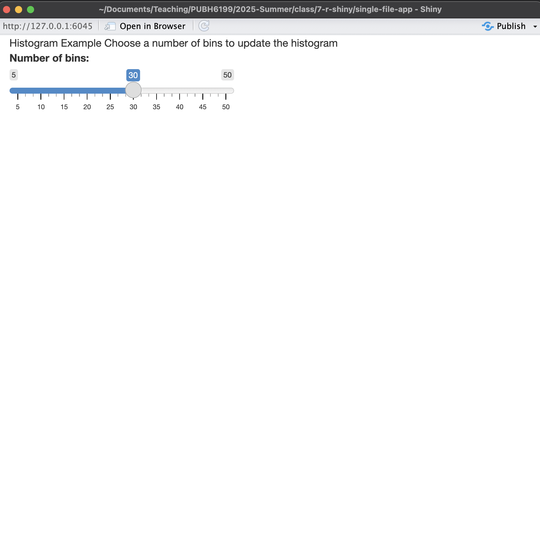
There is no distinction between title and subtitle
There is no plot

Adding hierarchy to the text

ui <- fluidPage(
  # app title
  h1("Histogram Example"),
  # app subtitle
  h4(strong("Choose a number of bins to update the histogram")),
  # slider input
  sliderInput("bins",
              "Number of bins:",
              min = 5, max = 50, value = 30),
  # histogram output
  plotOutput("histPlot")
)

Plot placeholder is present

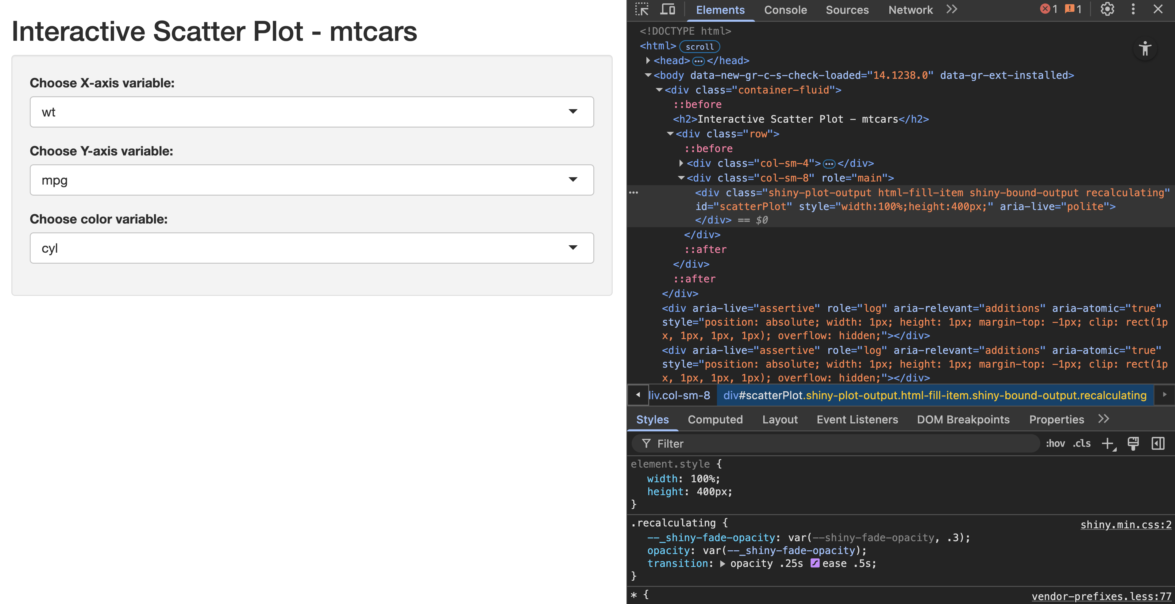
When developing with R shiny, it is recommended that you use Google Chrome browser, and learn how to inspect html pages by right-clicking on the page and selecting “Inspect” or pressing Ctrl + Shift + I (Windows/Linux) or Cmd + Option + I (Mac).

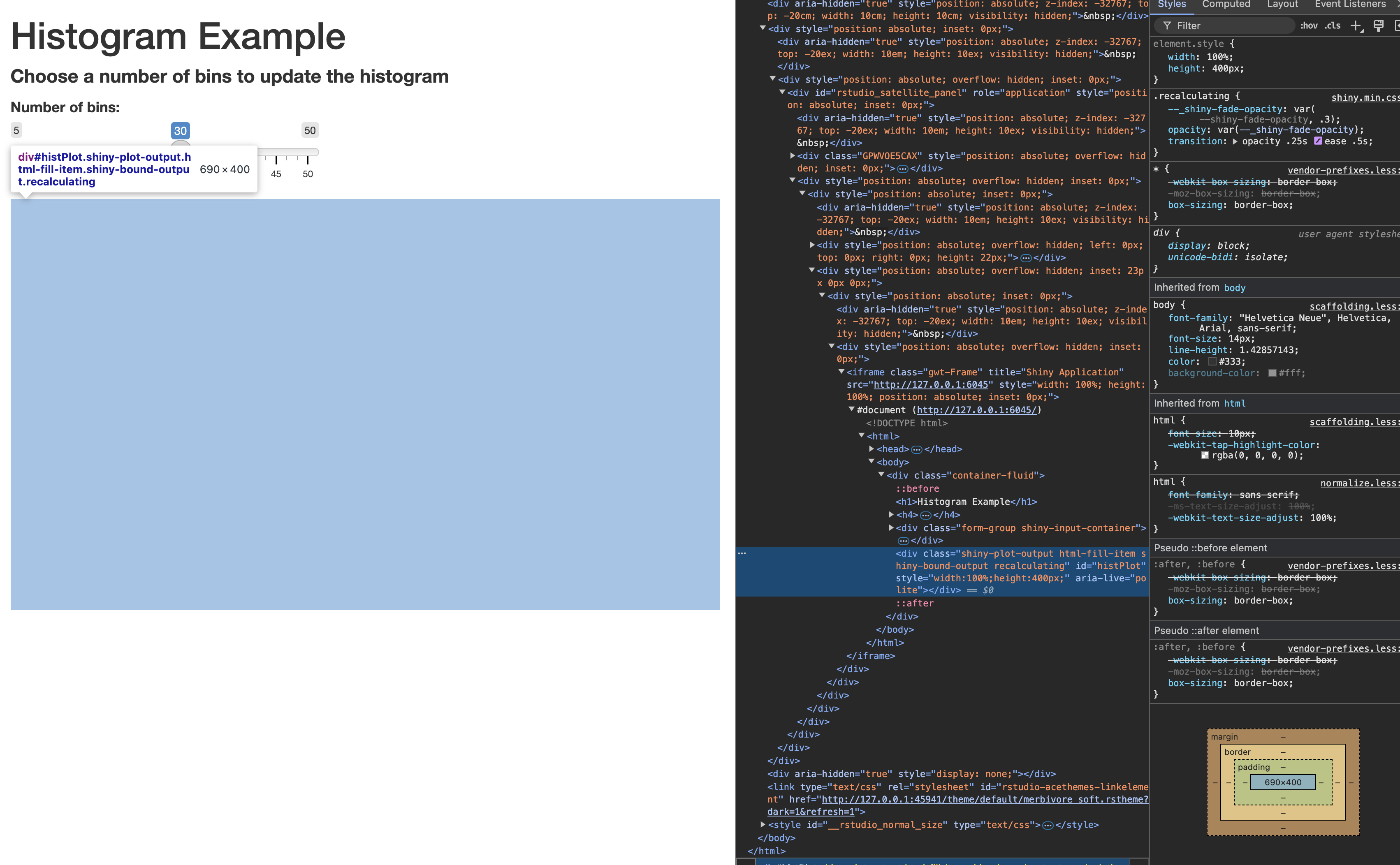
But the plot is not there yet, we need to add the server logic to create the plot.

Code Breakdown: Server

Server takes the inputs and create a reactive chart

server <- function(input, output) {
  
  output$histPlot <- renderPlot({
    # Generate random data
    data <- rnorm(500)
    
    # Create histogram with user-specified bins
    hist(data, breaks = 30, col = "skyblue",
         border = "white", main = "Histogram of Random Normal Data",
         xlab = "Value", ylab = "Frequency")
  })
}

shinyApp(ui = ui, server = server)

Running the App

Save the code to an R script file, e.g., app.R.
In your R console, run shiny::runApp("app.R")

How to make it reactive?

This will not react to user input because the number of bins is always 30.

server <- function(input, output) {
  output$histPlot <- renderPlot({
    # Generate random data
    data <- rnorm(500)
    # Create histogram with user-specified bins
    hist(data, breaks = 30, col = "skyblue",
         border = "white", main = "Histogram of Random Normal Data",
         xlab = "Value", ylab = "Frequency")
  })
}

shinyApp(ui = ui, server = server)

This takes in user input and uses it to create a histogram with the specified number of bins.

server <- function(input, output) {
  output$histPlot <- renderPlot({
    # Generate random data
    data <- rnorm(500)
    # Create histogram with user-specified bins
    hist(data, breaks = input$bins, col = "skyblue",
         border = "white", main = "Histogram of Random Normal Data",
         xlab = "Value", ylab = "Frequency")
  })
}

shinyApp(ui = ui, server = server)

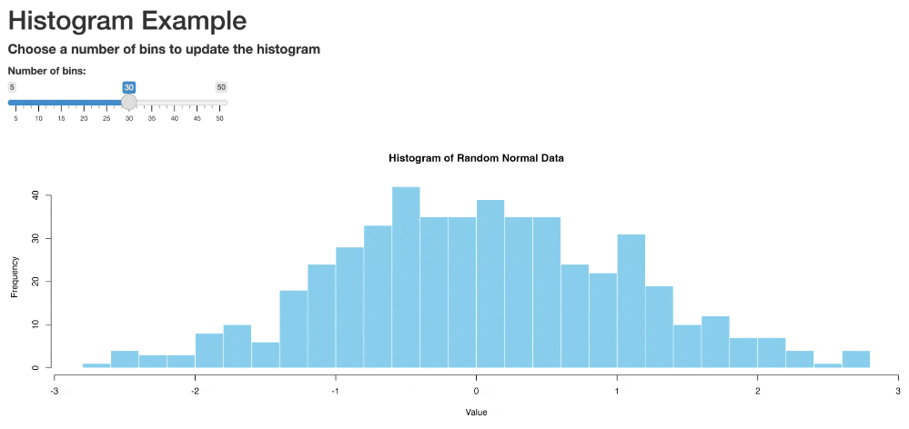
This is what we have now

ui <- fluidPage(
  # app title
  h1("Histogram Example"),
  # app subtitle
  h4(strong("Choose a number of bins to update the histogram")),
  # slider input
  sliderInput("bins",
              "Number of bins:",
              min = 5, max = 50, value = 30),
  # histogram output
  plotOutput("histPlot")
)

# Server
server <- function(input, output) {

  output$histPlot <- renderPlot({
    # Generate random data
    data <- rnorm(500)

    # Create histogram with user-specified bins
    hist(data, breaks = input$bins, col = "skyblue",
         border = "white", main = "Histogram of Random Normal Data",
         xlab = "Value", ylab = "Frequency")
  })
}

# Run the app
shinyApp(ui = ui, server = server)

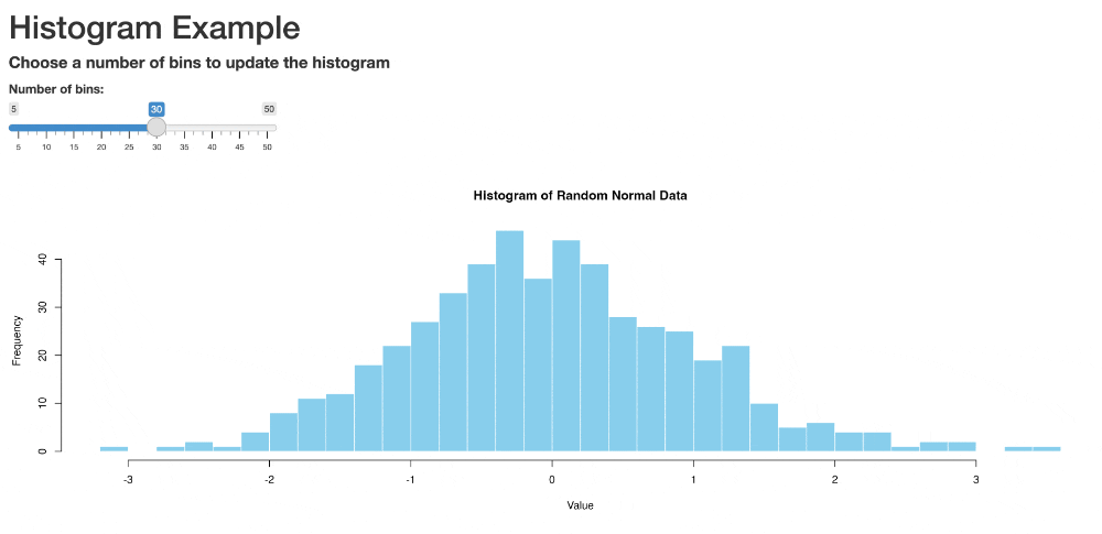
Adding visual structures

ui <- fluidPage(
  titlePanel("Histogram Example"),
  h4(strong("Choose a number of bins to update the histogram")),
  
  sidebarLayout(
    sidebarPanel(
      sliderInput("bins",
                  "Number of bins:",
                  min = 5, max = 50, value = 30)
    ),

    mainPanel(
      plotOutput("histPlot")
    )
  )
)

# Server
server <- function(input, output) {

  output$histPlot <- renderPlot({
    # Generate random data
    data <- rnorm(500)

    # Create histogram with user-specified bins
    hist(data, breaks = input$bins, col = "skyblue",
         border = "white", main = "Histogram of Random Normal Data",
         xlab = "Value", ylab = "Frequency")
  })
}

# Run the app
shinyApp(ui = ui, server = server)

In-Class Activity:

Add a second slider input so that the app reacts to the number of random data points generated for the histogram.

10:00

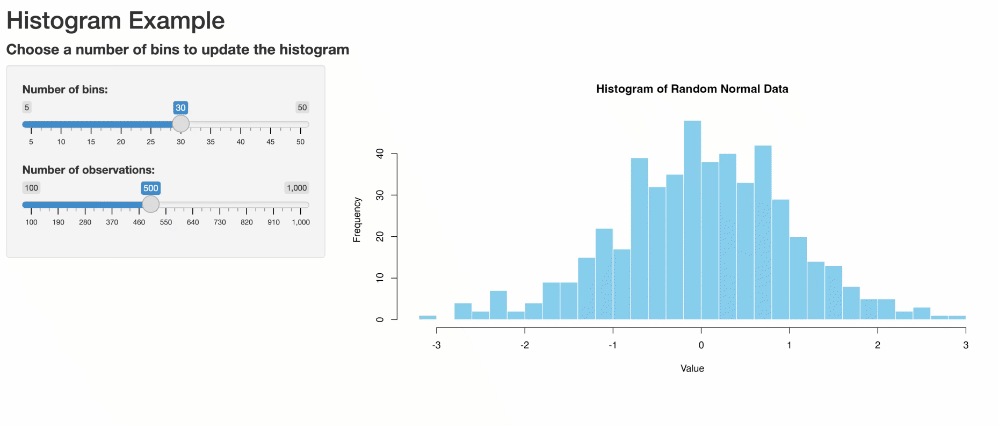
Finished app with two slider inputs

Two-file shiny app with a dataset

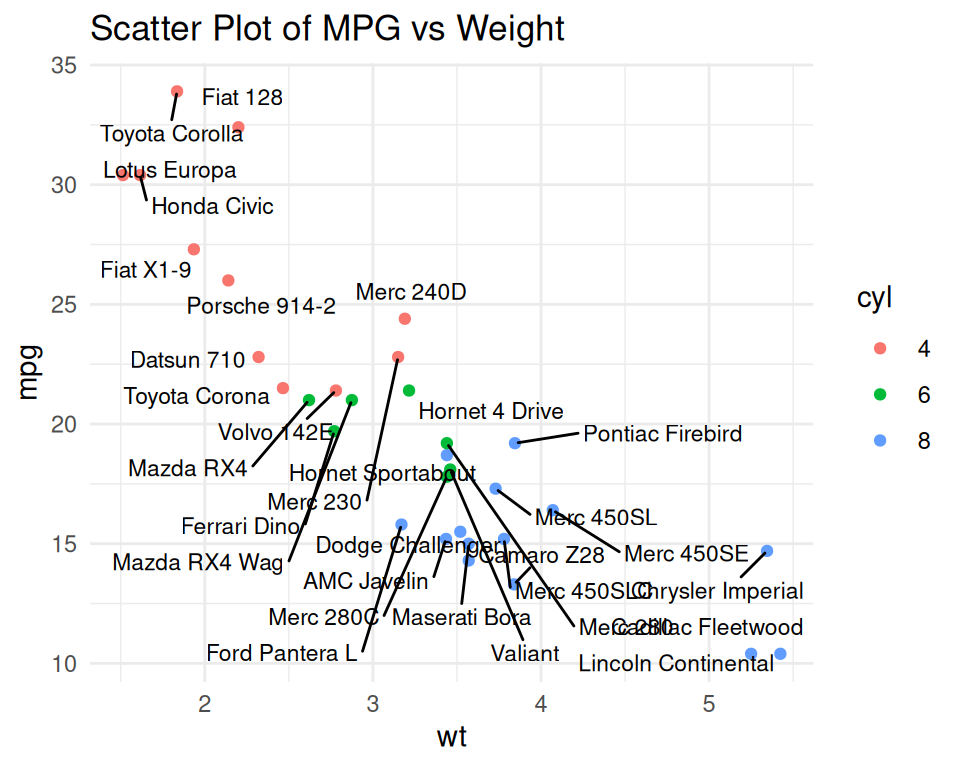
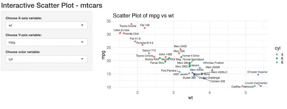
In this tutorial, we will build an interactive R Shiny application step-by-step. Our app will:

Display a scatter plot using the mtcars dataset
Allow users to choose x-axis and y-axis variables
Enable plot color customization by a third variable
Label points with car names

`global.R`: load libraries, clean data

library(shiny)
library(ggplot2)
library(dplyr)

# Data wrangling: Add a car name column and factor variables
mtcars_clean <- mtcars %>%
  tibble::rownames_to_column("car") %>%
  mutate(
    cyl = as.factor(cyl),
    gear = as.factor(gear)
  )
glimpse(mtcars_clean)

Rows: 32
Columns: 12
$ car  <chr> "Mazda RX4", "Mazda RX4 Wag", "Datsun 710", "Hornet 4 Drive", "Ho…
$ mpg  <dbl> 21.0, 21.0, 22.8, 21.4, 18.7, 18.1, 14.3, 24.4, 22.8, 19.2, 17.8,…
$ cyl  <fct> 6, 6, 4, 6, 8, 6, 8, 4, 4, 6, 6, 8, 8, 8, 8, 8, 8, 4, 4, 4, 4, 8,…
$ disp <dbl> 160.0, 160.0, 108.0, 258.0, 360.0, 225.0, 360.0, 146.7, 140.8, 16…
$ hp   <dbl> 110, 110, 93, 110, 175, 105, 245, 62, 95, 123, 123, 180, 180, 180…
$ drat <dbl> 3.90, 3.90, 3.85, 3.08, 3.15, 2.76, 3.21, 3.69, 3.92, 3.92, 3.92,…
$ wt   <dbl> 2.620, 2.875, 2.320, 3.215, 3.440, 3.460, 3.570, 3.190, 3.150, 3.…
$ qsec <dbl> 16.46, 17.02, 18.61, 19.44, 17.02, 20.22, 15.84, 20.00, 22.90, 18…
$ vs   <dbl> 0, 0, 1, 1, 0, 1, 0, 1, 1, 1, 1, 0, 0, 0, 0, 0, 0, 1, 1, 1, 1, 0,…
$ am   <dbl> 1, 1, 1, 0, 0, 0, 0, 0, 0, 0, 0, 0, 0, 0, 0, 0, 0, 1, 1, 1, 0, 0,…
$ gear <fct> 4, 4, 4, 3, 3, 3, 3, 4, 4, 4, 4, 3, 3, 3, 3, 3, 3, 4, 4, 4, 3, 3,…
$ carb <dbl> 4, 4, 1, 1, 2, 1, 4, 2, 2, 4, 4, 3, 3, 3, 4, 4, 4, 1, 2, 1, 1, 2,…

`ui.R`: define user interface

ui <- fluidPage(
  titlePanel("Interactive Scatter Plot - mtcars"),
  
  sidebarLayout(
    sidebarPanel(
      selectInput("xvar", "Choose X-axis variable:", choices = names(mtcars), selected = "wt"),
      selectInput("yvar", "Choose Y-axis variable:", choices = names(mtcars), selected = "mpg"),
      selectInput("colorvar", "Choose color variable:", choices = names(mtcars), selected = "cyl"),
    ),
    mainPanel(
      plotOutput("scatterPlot")
    )
  )
)

Intermediate step: make ggplot in `scratch.R`

This is not a must but highly recommend, you can test out your ggplot code in a separate R script file, e.g., scratch.R, before integrating it into the Shiny app.

ggplot(mtcars_clean, aes(x = wt, y = mpg)) +
  geom_point(aes(color = cyl)) +
  ggrepel::geom_text_repel(aes(label = car), vjust = -1, size = 3) +
  labs(
    title = "Scatter Plot of MPG vs Weight"
  ) +
  theme_minimal()

`server.R`: adapt regular ggplot code

scratch.R

ggplot(mtcars_clean, aes(x = wt, y = mpg)) +
  geom_point(aes(color = cyl)) +
  geom_text(aes(label = car), vjust = -1, size = 3) +
  labs(
    title = "Scatter Plot of MPG vs Weight"
  ) +
  theme_minimal()

Regular ggplot code for scatter plot
x-axis is wt
y-axis is mpg
color by cyl
label points with car names

server.R

server <- function(input, output) {
  # Render the plot
  output$scatterPlot <- renderPlot({
    ggplot(mtcars_clean, aes_string(x = input$xvar, y = input$yvar)) +
      geom_point(aes_string(color = input$colorvar), size = 3) +
      geom_text(aes(label = car), vjust = -1, size = 3) +
      theme_minimal() +
      labs(title = paste("Scatter Plot of", input$yvar, "vs", input$xvar),
           x = input$xvar, y = input$yvar)
  })
}

Adapt the ggplot code to use aes_string() for dynamic variable selection
Use input$xvar, input$yvar, and input$colorvar to make the plot reactive

Run the two-file Shiny app

No need for shinyApp(ui = ui, server = server) when you have two-file app structure:

Save the ui.R and server.R files in the same directory
Shiny automatically stitch them together, and optionally look for global.R.
In RStudio, click the Run App button

Outline for today

What is R Shiny
Write a basic R shiny app
Deploy your Shiny apps with shinyapps.io
AI-powered help: using Shiny Assistant

Why `shinyapps.io`?

Free: Free tier available for up to 5 small apps
Easy to use: No need to set up a server or manage infrastructure
Scalable: Can handle apps of varying sizes and complexities
Integration with RStudio: Seamless deployment from RStudio IDE

Getting started with `shinyapps.io`

Create an account on shinyapps.io
Recommended to log in using GitHub
Install the rsconnect package in R: install.packages("rsconnect")
Following the instructions on the shinyapps.io to authorize your account

Deploy your app to `shinyapps.io`

In RStudio, open the app you want to deploy
Click on the Publish button in the top right corner of the RStudio IDE
Select the shinyapps.io account you just connected
Fill in the app name and description
Click Publish to deploy your app
Once deployed, a browser will open to your application. https://{your-username}.shinyapps.io/{your-app-directory-name}
You should see a rsconnect/ folder within your app directory, which contains the deployment information. This should be added and committed into version control (i.e. push it to GitHub)

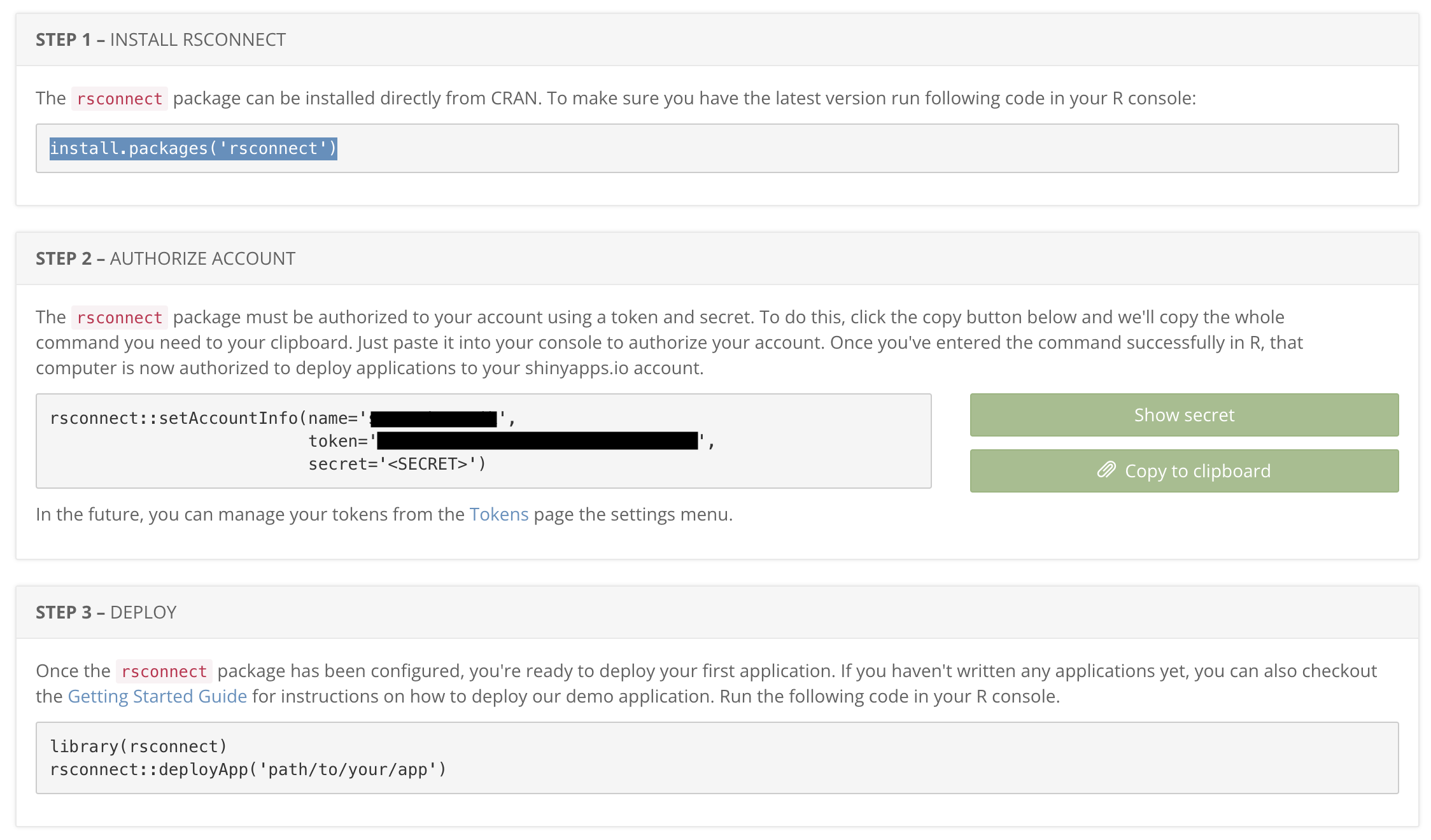
`shinyapps.io` dashboard

Dashboard provides an overview of your deployed apps, including: app name and URL, deployment status, usage statistics (e.g., number of active users, CPU usage)

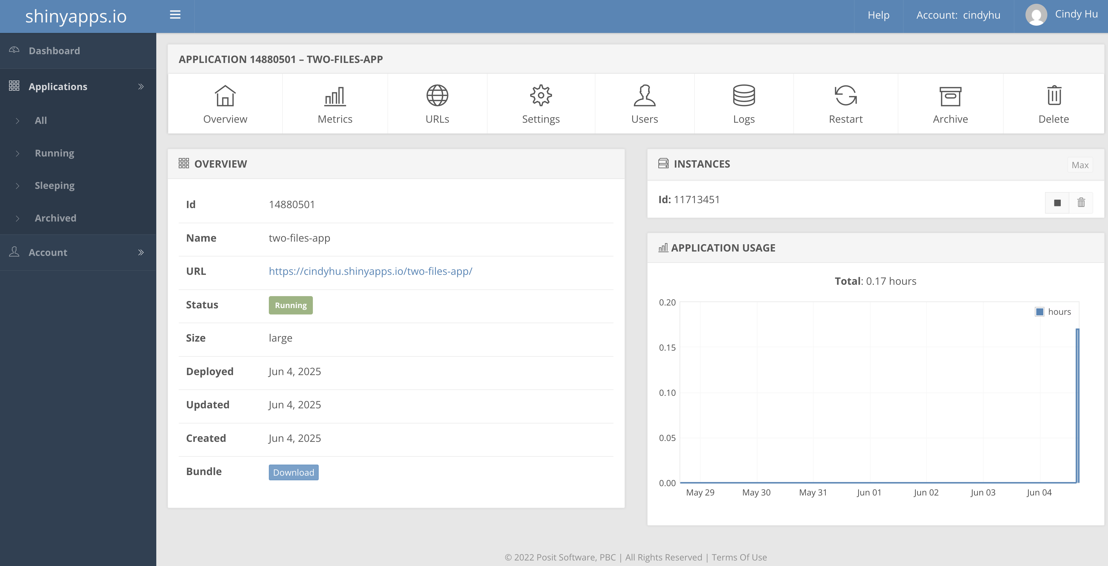
Check out shinyapps.io user guide for more information on hosting your app!

Outline for today

What is R Shiny
Write a basic R shiny app
Deploy your Shiny apps with shinyapps.io
AI-powered help: using Shiny Assistant

What is Shiny Assistant?

https://gallery.shinyapps.io/assistant/

Use Shiny Assistant to recreate the two-file shiny app

Prompt: Create a shiny app using the mtcars dataset. Use three files global.R, ui.R, server.R. The app displays an interactive scatter plot that reacts to user input of x-axis, y-axis, and a third variable for color of the points. Show car name as label text next to the points.

Next, let’s build a `shinydashboard`

The {shinydashboard} package provides a framework for building dashboards in R Shiny. It allows you to create visually appealing and interactive apps with a more classic “dashboard” layout, including sidebars, tabs, and boxes. You need both packages: {shiny} and {shinydashboard}.

Use Shiny Assistant to create a `shinydashboard`

Prompt: Create a shinydashboard using the mtcars dataset. Use three files global.R, ui.R, server.R. The app allows users to filter by mpg and displays three output: an interactive scatter plot that reacts to user input of x-axis, y-axis, and color variable. A heatmap of car performance. And a data table of the filtered dataset. Show car name as label text next to the points in the scatter plot.

Refine the app locally

Download the code from Shiny Assistant
Save the files in your local R project directory, remember to organize your repo structure well
Open the files in RStudio and run the app locally
Make any necessary adjustments to the code

Your turn in `hw4`

Try one of these built-in datasets to explore with Shiny Assistant

Dataset	Description
`mtcars` 🚗	Car performance data (mpg, cylinders, hp)
`iris` 🌸	Iris flower measurements (sepal, petal, species)
`diamonds` 💎	Diamond pricing (carat, cut, price, etc.)
`faithful` 🌋	Old Faithful geyser eruptions (duration, waiting time)
`airquality` 🌍	New York air quality data (Ozone, Temp, Wind)
`ToothGrowth` 🦷	Vitamin C & tooth growth in guinea pigs

Or upload your own dataset to GitHub and give Shiny Assistant a public URL!

Write good prompt, and you will get good code!

Describe what change you made to the app on top of what Shiny Assistant generated.

Further resources

How much time do you have?

10 min: Print out this Shiny for R cheatsheet
2.5 hrs: Follow this Posit tutorial
Lifetime: Check out resources like the Shiny Gallery, TidyTuesday, and Mastering Shiny book
Unknown: chatGPT, Gemini, Shiny Assistant (powered by Anthropic), and other AI tools can help you build Shiny apps

End-of-Class Survey

Fill out the end-of-class survey

~ This is the end of Lecture 4 ~

10:00

Lecture 4.Introduction to R Shiny

Outline for today

About R Shiny

Key Features

Basic Structure Shiny Application

Visual Logic

*Input(), *Output() and render*()

*Input() function syntax

Different types of UI Inputs

*Output() function syntax

Output <-> Render pairing

Outline for today

Setting up a shiny app

Two options for shiny apps

Create a single-file Shiny app

Let’s build the app step-by-step

Code Breakdown UI

UI Work-in-Progress

Adding hierarchy to the text

Plot placeholder is present

Code Breakdown: Server

Running the App

How to make it reactive?

This is what we have now

Adding visual structures

Finished app with two slider inputs

Two-file shiny app with a dataset

global.R: load libraries, clean data

ui.R: define user interface

Intermediate step: make ggplot in scratch.R

server.R: adapt regular ggplot code

Run the two-file Shiny app

Outline for today

Why shinyapps.io?

Getting started with shinyapps.io

Deploy your app to shinyapps.io

shinyapps.io dashboard

Outline for today

What is Shiny Assistant?

Use Shiny Assistant to recreate the two-file shiny app

Next, let’s build a shinydashboard

Use Shiny Assistant to create a shinydashboard

Refine the app locally

Your turn in hw4

Further resources

End-of-Class Survey

`Input()`, `Output()` and `render*()`

`*Input()` function syntax

`*Output()` function syntax

`global.R`: load libraries, clean data

`ui.R`: define user interface

Intermediate step: make ggplot in `scratch.R`

`server.R`: adapt regular ggplot code

Why `shinyapps.io`?

Getting started with `shinyapps.io`

Deploy your app to `shinyapps.io`

`shinyapps.io` dashboard

Next, let’s build a `shinydashboard`

Use Shiny Assistant to create a `shinydashboard`

Your turn in `hw4`