Lecture 5. Maps
PUBH 6199: Visualizing Data with R, Summer 2025
2025-06-17
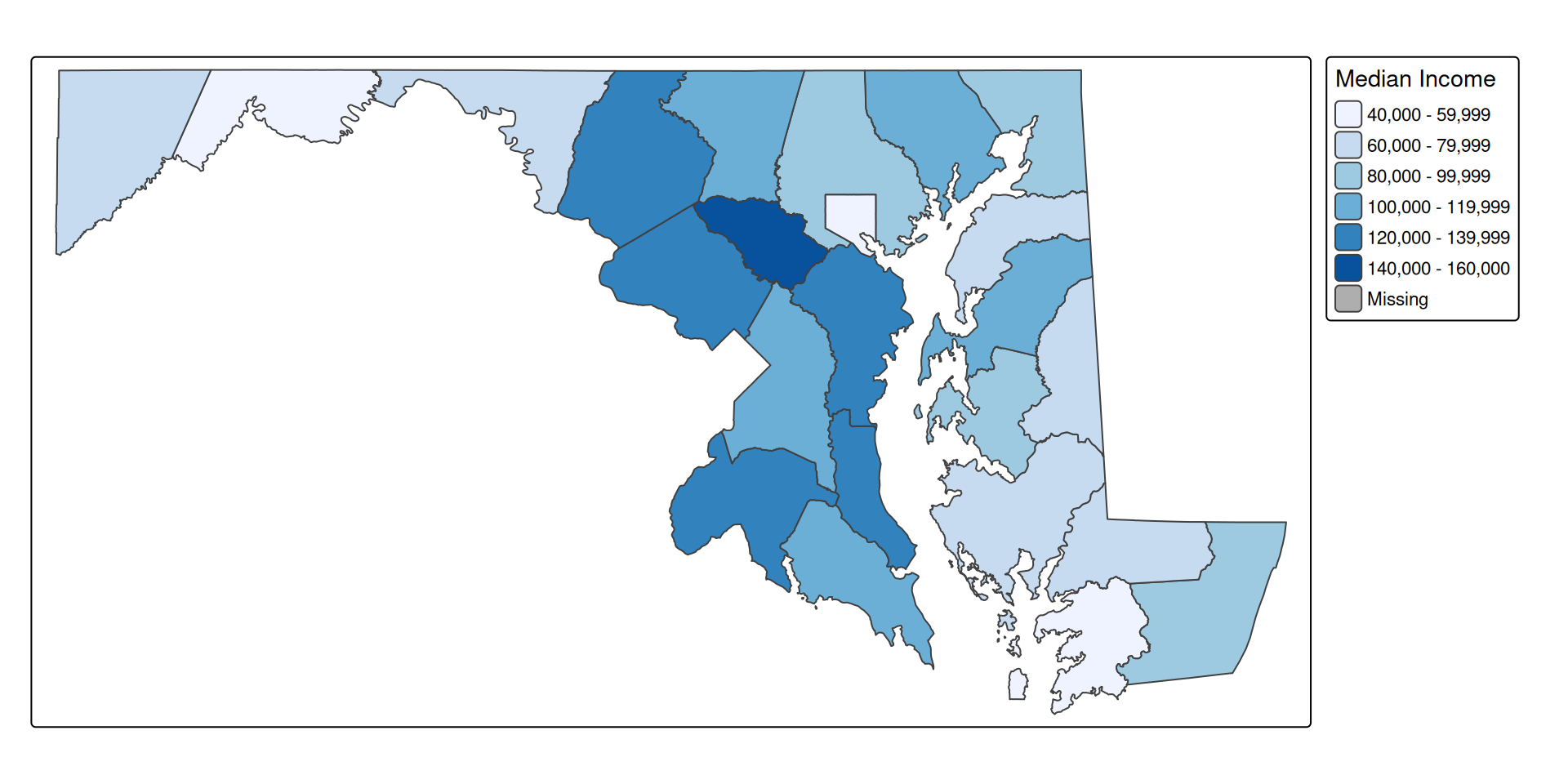
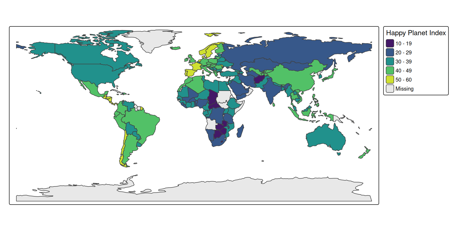
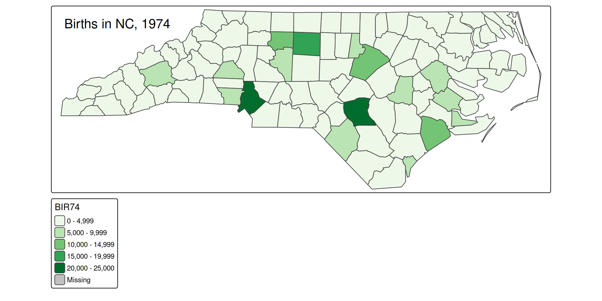
Example: Choropleth
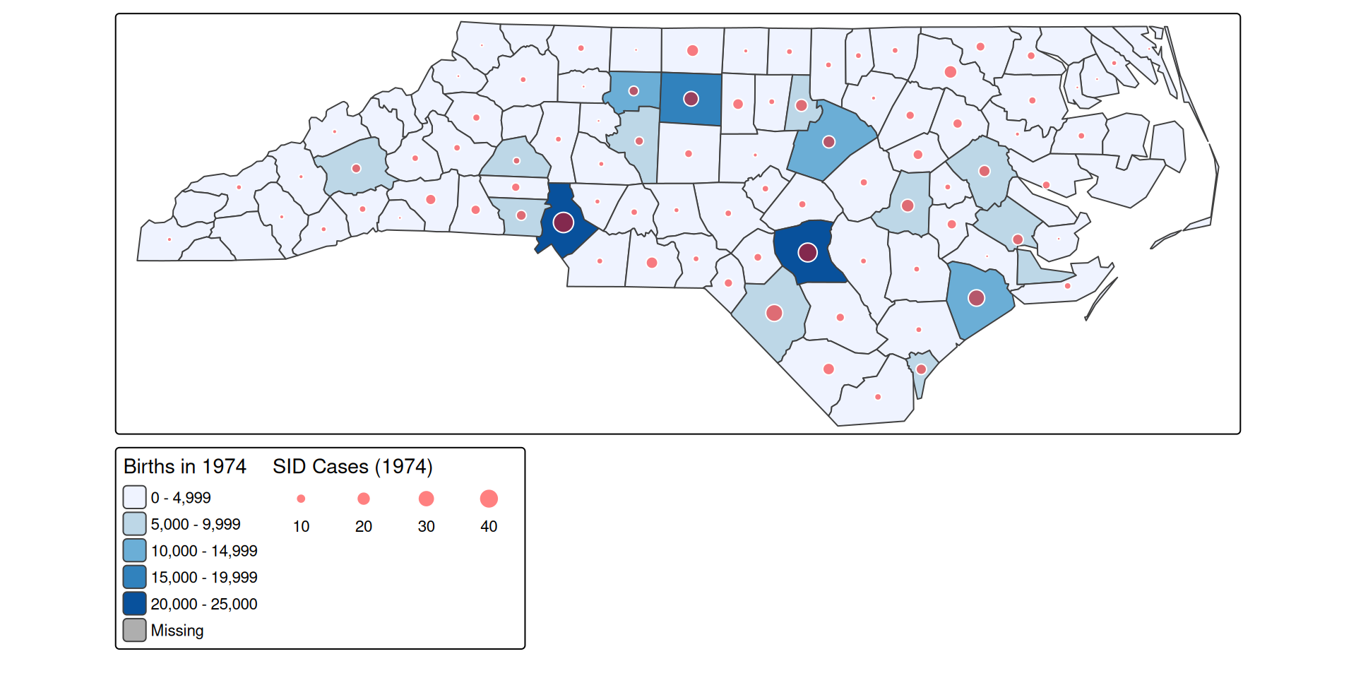
Example: Point Map
library(tidyverse)
library(spData)
library(tmap)
data(urban_agglomerations)
urb_2030 <- urban_agglomerations |> filter(year == 2030)
tm_shape(World) +
  tm_polygons() +
  tm_shape(urb_2030) +
  tm_symbols(fill = "black", col = "white", size = "population_millions",
             size.legend = tm_legend(title = "Urban Population in 2030\n(millions)"))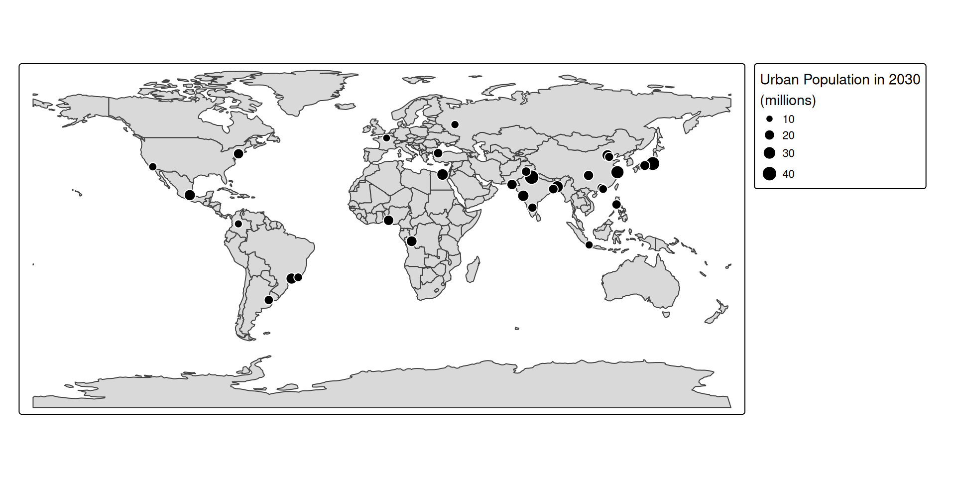
Example: Faceted Map
library(tidyverse)
library(spData)
library(tmap)
data(urban_agglomerations)
urb_1970_2030 <- urban_agglomerations |> filter(year %in% c(1970, 1990, 2010, 2030))
tm_shape(World) +
  tm_polygons() +
  tm_shape(urb_1970_2030) +
  tm_symbols(fill = "black", col = "white", size = "population_millions",
             size.legend = tm_legend(title = "Urban Population\n(millions)")) +
  tm_facets(by = "year", ncol = 2)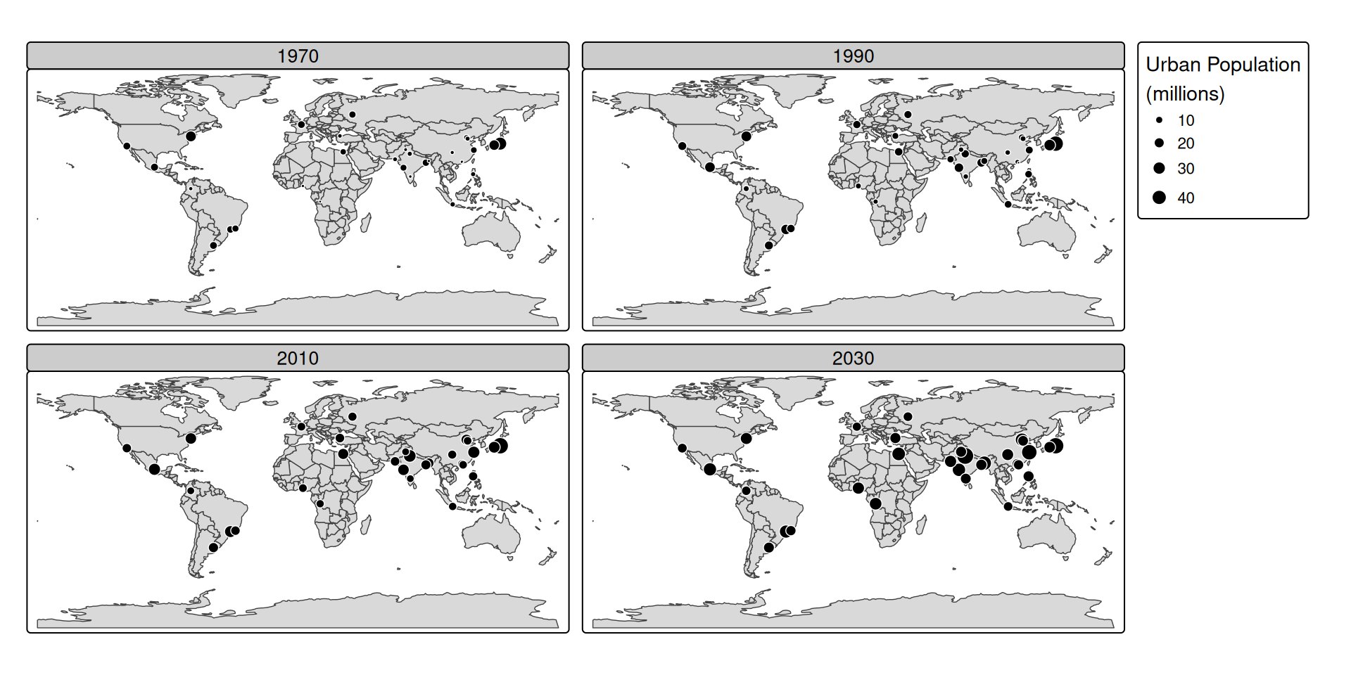
Color Choices for Maps
- Sequential palettes for ordered values
- Diverging palettes for above/below mean
- Qualitative for categories
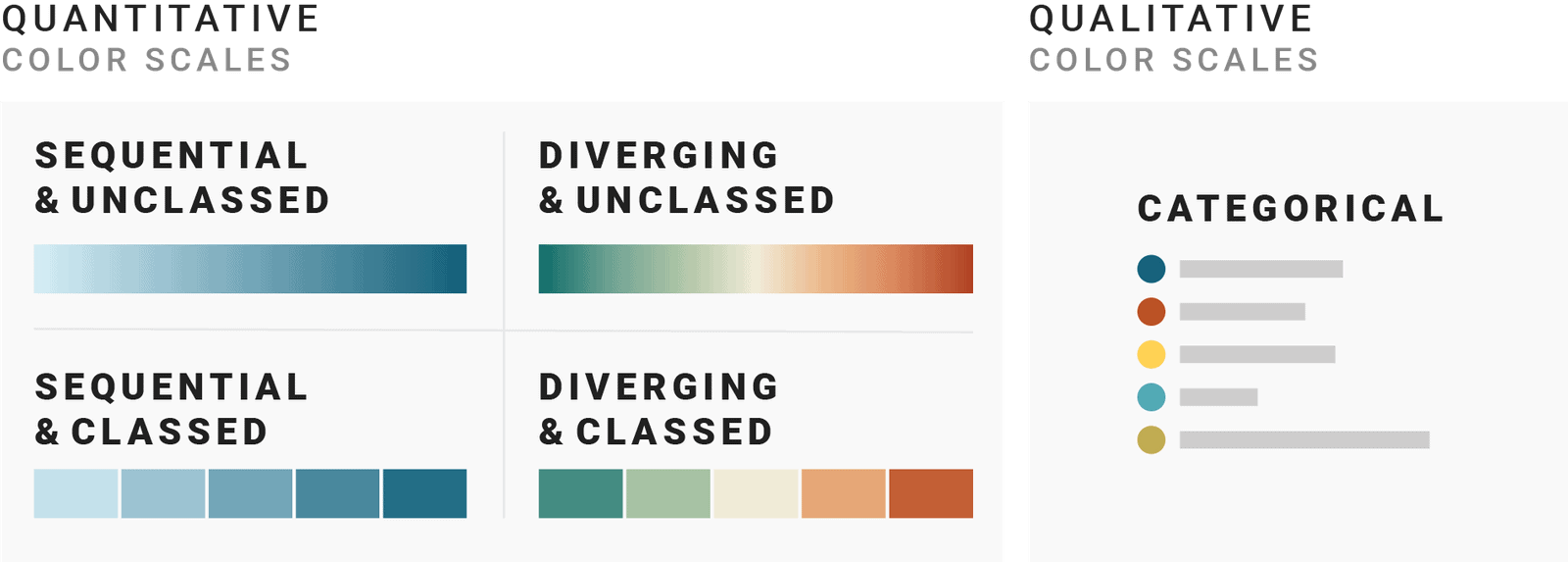
Source: Which color scale to use when visualizing data, by Lisa Charlottte Muth.
Categorical scales
- Use distinct hues for different categories
- Limit to no more than 7 hues
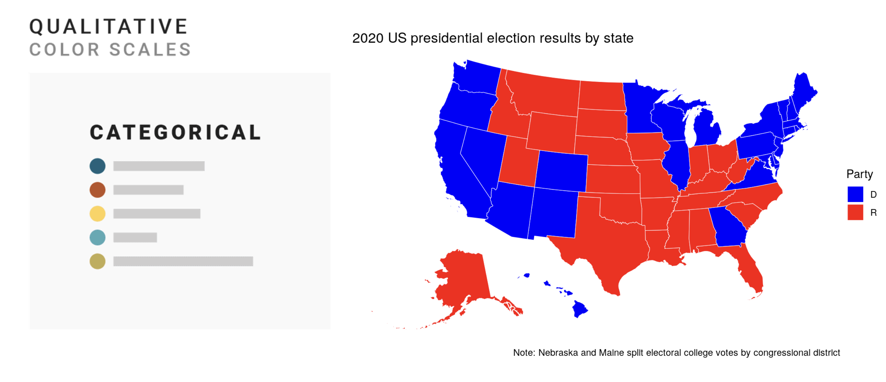
Source: Analyzing US Census Data, by Kyle Walker
Sequential Scales
- Map value to color on a continuum, based on both intensity and hue
- Use for ordered data (e.g., population, income)
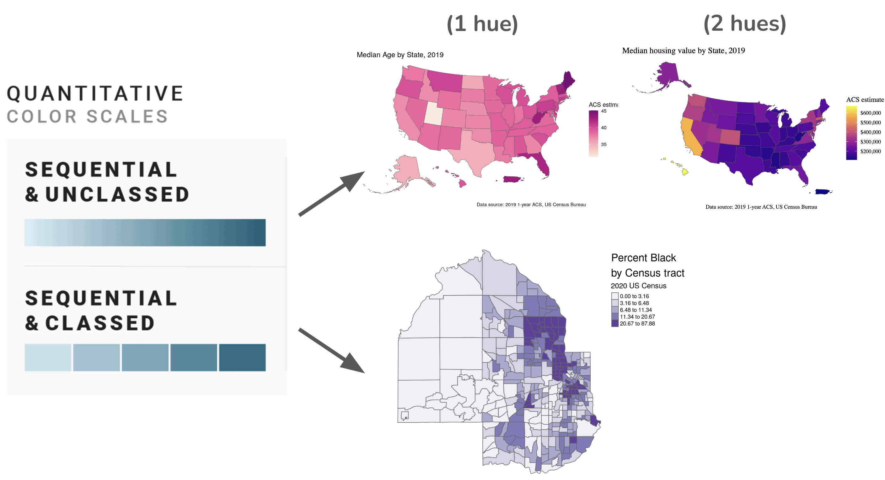
Source: Analyzing US Census Data, by Kyle Walker
Diverging Scales
- Use for data with a meaningful midpoint (e.g., above/below average)
- Two contrasting colors with a neutral midpoint (e.g., white/light gray)
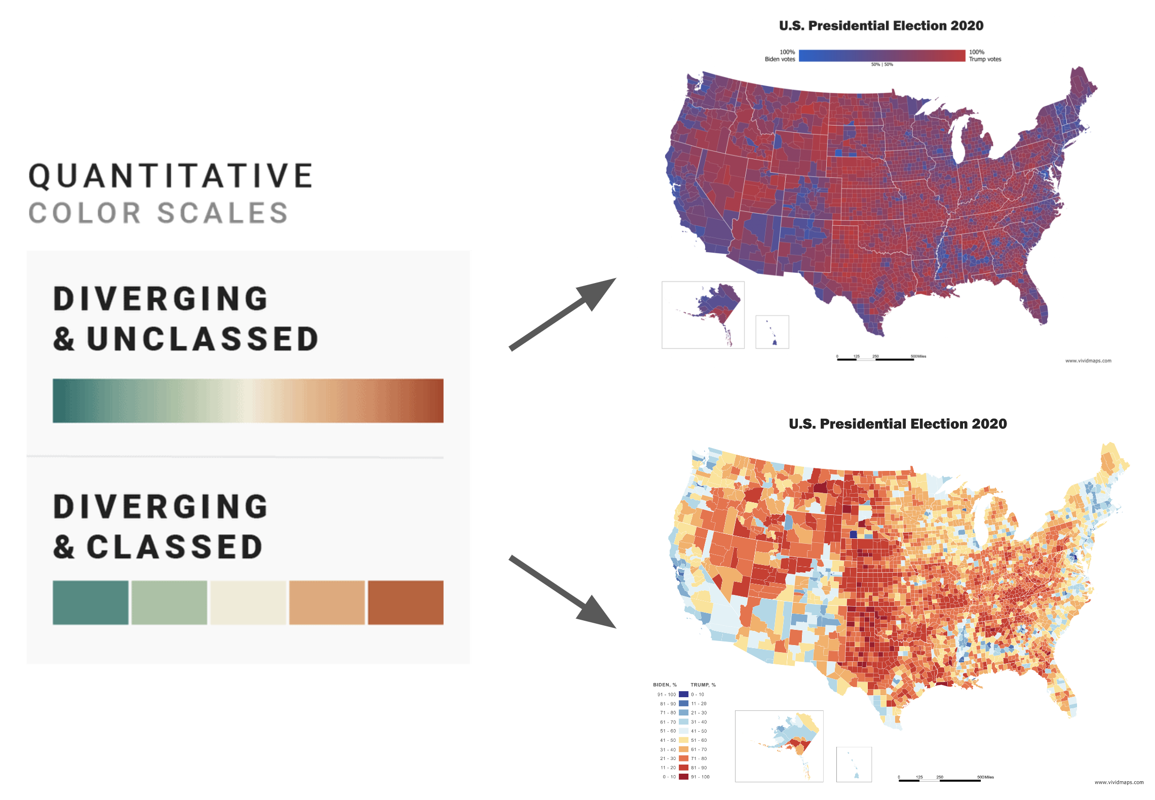
Source: 2020 U.S. Election Mapped, by Vivid Maps
Avoid Misleading Colors
- Don’t use rainbow: not perceptually uniform
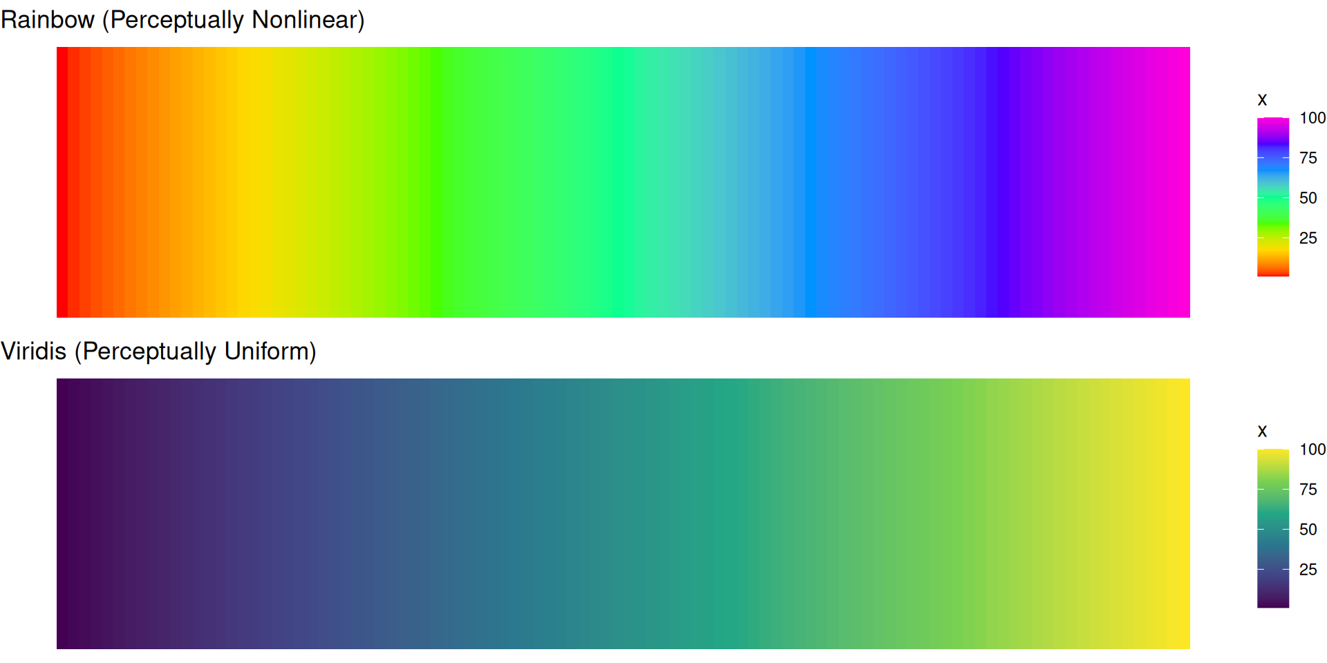
- Consider accessibility (color-blind safe palettes)
- Avoid encoding meaning with non-intuitive colors
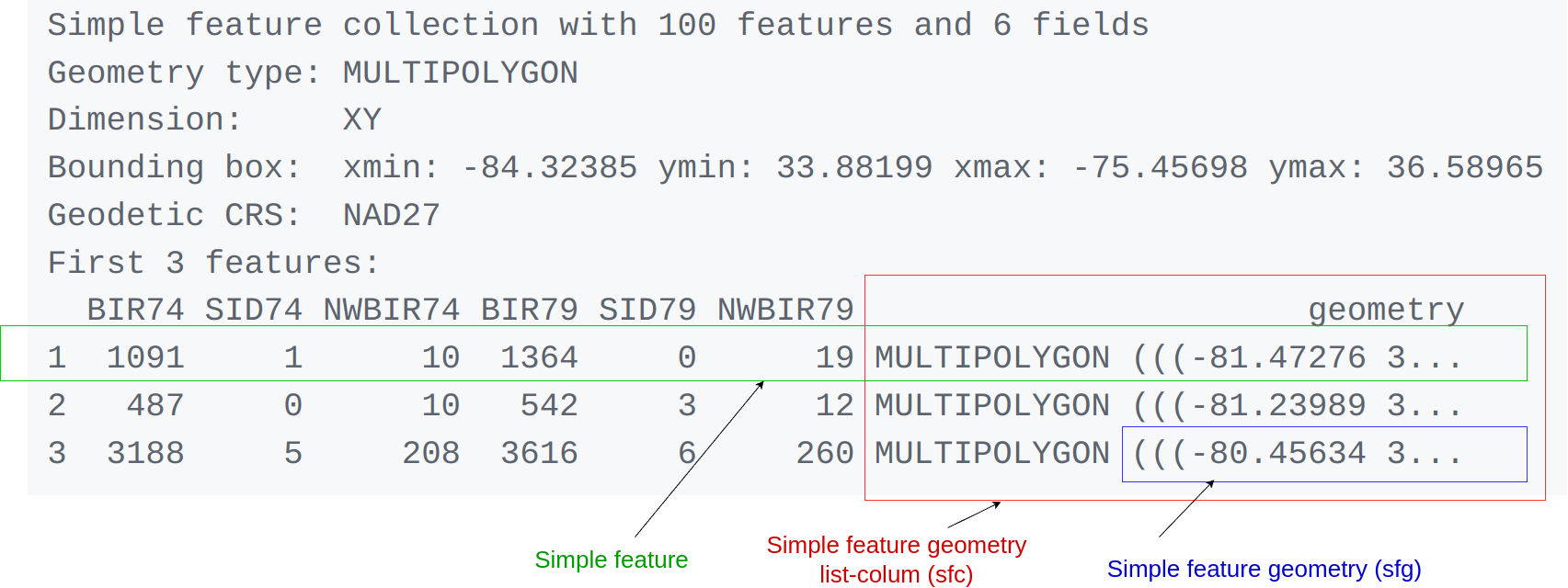
{sf}: simple features
The {sf} package is the standard way to work with vector spatial data in R. It replaces older tools like {sp} with a simple, tidy-friendly interface.
Key Features of {sf}
- Stores geometry + attributes in a single
data.frame-like object - Built on simple features standard (ISO 19125-1)
- Fully compatible with
dplyr,ggplot2,tmap - Uses
sfccolumn to store spatial information (e.g., points, polygons)
Static Mapping with tmap
- Similar to
ggplot2, based on “the grammar of graphics” - Supports both static and interactive modes
- Excellent for quick, polished maps, sensible defaults
Adding layers in {tmap}
tm_polygons(): for choropleth mapstm_symbols(): for point data, size and color can represent different variables
Scale
Scales control how the values are represented on the map and in the legend, and can have a major impact on how spatial variability is portrayed
tm_shape(nz) + tm_polygons(fill = "Median_income")
tm_shape(nz) + tm_polygons(fill = "Median_income",
                        fill.scale = tm_scale(breaks = c(0, 30000, 40000, 50000)))
tm_shape(nz) + tm_polygons(fill = "Median_income",
                           fill.scale = tm_scale(n = 10))
tm_shape(nz) + tm_polygons(fill = "Median_income",
                           fill.scale = tm_scale(values = "BuGn"))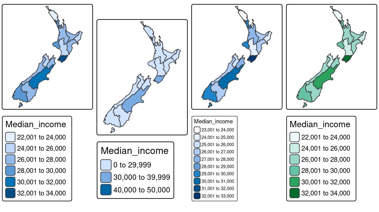
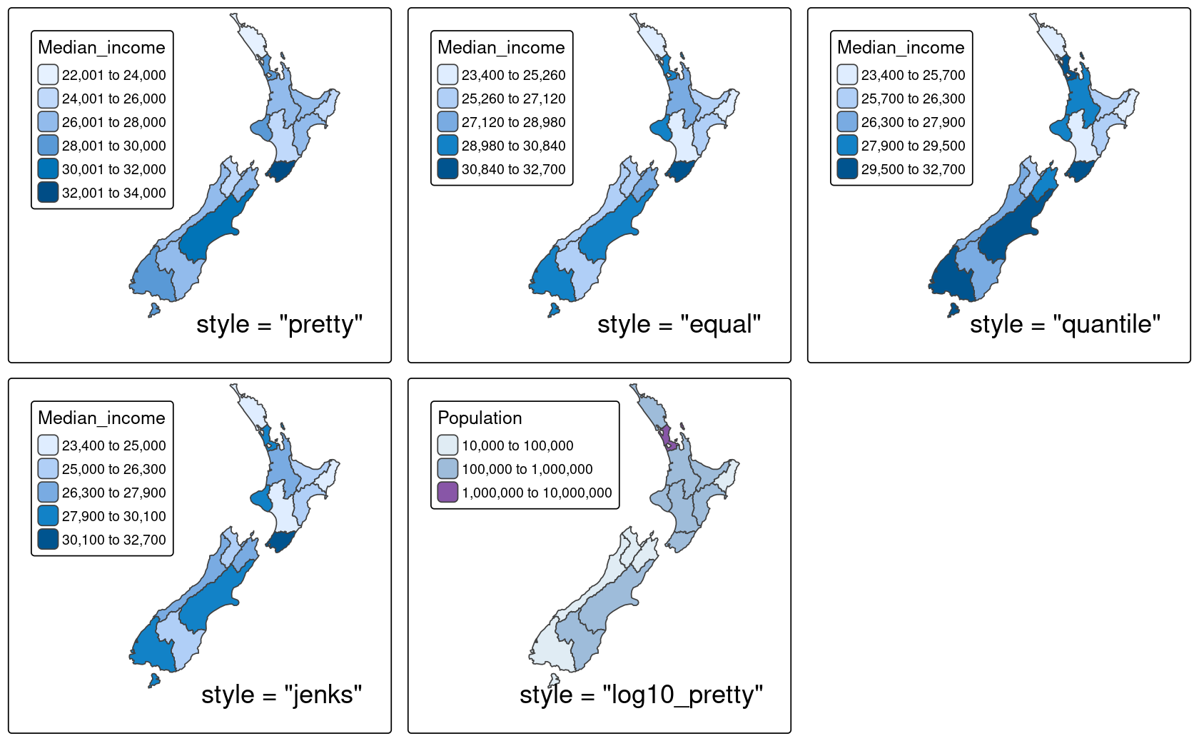
Style options for classifying map data
tm_scale_intervals(style = "pretty"):
- “pretty”: Rounded, evenly spaced breaks (default).
- “equal”: Equal-width bins; poor fit for skewed data — may hide variation.
- “quantile”: Equal count per bin; be careful with wide bin ranges.
- “jenks”: Optimizes natural groupings; can be slow with large datasets.
- “log10_pretty”: Log-scaled breaks; only appropriate for right-skewed, positive values.
Getting Data with tigris
The
{tigris}package provides access to U.S. Census Bureau geographic data. Shapefiles downloaded using {tigris} will be loaded as a simple features (sf) object with geometries.
A shapefile is a vector data file format commonly used for geospatial analysis.
Shapefiles contain information for spatially describing features (e.g. points, lines, polygons), as well as any associated attribute information.
You can find / download shapefiles online (e.g. from the US Census Bureau), or depending on the tools available, access them via packages (like we’re doing today).
Plotting Census Data